pyCropWat

A Python Package for Computing Effective Precipitation Using Google Earth Engine Climate Data.

pyCropWat Logo

Project Structure

pyCropWat/
├── pycropwat/               # Main package
│   ├── __init__.py          # Package exports
│   ├── core.py              # EffectivePrecipitation class
│   ├── methods.py           # Effective precipitation methods (9 methods)
│   ├── analysis.py          # Temporal aggregation, statistics, visualization
│   ├── utils.py             # Utility functions (geometry loading, GEE init)
│   └── cli.py               # Command-line interface
├── tests/                   # Unit tests
│   ├── __init__.py
│   └── test_core.py
├── docs/                    # MkDocs documentation
│   ├── index.md             # Documentation home
│   ├── installation.md      # Installation guide
│   ├── examples.md          # Usage examples
│   ├── contributing.md      # Contribution guidelines
│   ├── assets/              # Documentation assets
│   │   ├── pyCropWat.png    # Logo image
│   │   ├── pyCropWat.gif    # Animated logo
│   │   ├── pyCropWat_logo.png  # Alternative logo
│   │   └── examples/        # Example output images for docs
│   │       ├── arizona/     # Arizona example figures
│   │       ├── comparisons/ # Dataset comparison figures
│   │       ├── figures/     # Rio de la Plata figures
│   │       ├── method_comparison/  # Method comparison figures
│   │       ├── new_mexico/  # New Mexico example figures
│   │       └── pcml/        # Western U.S. PCML example figures
│   ├── api/                 # API reference
│   │   ├── analysis.md
│   │   ├── cli.md
│   │   ├── core.md
│   │   ├── methods.md
│   │   └── utils.md
│   └── user-guide/          # User guide
│       ├── api.md
│       ├── cli.md
│       └── quickstart.md
├── Examples/                # Example scripts and data
│   ├── README.md                  # Detailed workflow documentation
│   ├── south_america_example.py   # Rio de la Plata workflow script
│   ├── arizona_example.py         # Arizona workflow script
│   ├── new_mexico_example.py      # New Mexico workflow script
│   ├── western_us_pcml_example.py # Western U.S. PCML workflow script
│   ├── ucrb_example.py            # UCRB field-scale workflow script
│   ├── AZ.geojson                 # Arizona boundary GeoJSON
│   ├── NM.geojson                 # New Mexico boundary GeoJSON
├── .github/                 # GitHub configuration
│   └── workflows/
│       ├── docs.yml         # GitHub Pages deployment workflow
│       └── publish.yml      # PyPI publishing workflow
├── CHANGELOG.md             # Release notes
├── MANIFEST.in              # PyPI package manifest
├── mkdocs.yml               # MkDocs configuration
├── environment.yml          # Conda environment file
├── pyproject.toml           # Package configuration
├── requirements.txt         # pip dependencies
├── LICENSE
└── README.md

Note: The Examples/ folder contains complete workflow scripts with detailed documentation in README.md.

south_america_example.py: A comprehensive Python script demonstrating the complete pyCropWat workflow including data processing, temporal aggregation, statistical analysis, visualization (including anomaly, climatology, and trend maps), and dataset comparison using real Rio de la Plata data.
arizona_example.py: A U.S.-focused workflow demonstrating 8 Peff methods with GridMET/PRISM precipitation and SSURGO AWC for Arizona, with U.S. vs Global dataset comparisons (excludes PCML).
new_mexico_example.py: A New Mexico workflow comparing 8 Peff methods using PRISM precipitation with SSURGO AWC and gridMET ETo (excludes PCML).
AZ.geojson: Arizona boundary GeoJSON for local geometry support.
NM.geojson: New Mexico boundary GeoJSON for local geometry support.

Note: Output rasters (~32 GB) are not included in the repository. Run the example scripts with a GEE project ID to generate them locally.

See the Complete Workflow Examples section below for details.

Changelog: See CHANGELOG.md for release notes and version history.

Overview

pyCropWat converts precipitation data from any GEE climate dataset into effective precipitation and effective precipitation fraction rasters. It supports:

Any GEE ImageCollection with precipitation data from the GEE Data Catalog or Community Catalog
Shapefile, GeoJSON, or GEE FeatureCollection asset for region of interest
Multiple effective precipitation methods: CROPWAT, FAO/AGLW, Fixed Percentage, Dependable Rainfall, FarmWest, USDA-SCS, TAGEM-SuET, PCML, Ensemble
Parallel processing using Dask
Monthly output rasters in GeoTIFF format
Temporal aggregation: Seasonal, annual, growing season (with cross-year support for Southern Hemisphere), custom date ranges
Statistical analysis: Climatology, anomalies, trend analysis
Enhanced exports: NetCDF, Cloud-Optimized GeoTIFF (COG), zonal statistics CSV
Visualization: Time series plots, maps, climatology charts, anomaly maps, trend maps with significance

Effective Precipitation Methods

pyCropWat supports multiple methods for calculating effective precipitation:

Method	Description
`cropwat`	CROPWAT method from FAO
`fao_aglw`	FAO/AGLW Dependable Rainfall (80% exceedance)
`fixed_percentage`	Simple fixed percentage method (configurable, default 70%)
`dependable_rainfall`	FAO Dependable Rainfall at specified probability level
`farmwest`	FarmWest method: Peff = (P - 5) × 0.75
`usda_scs`	USDA-SCS method with AWC and ETo (requires GEE assets)
`suet`	TAGEM-SuET method: P - ETo with 75mm threshold (requires ETo asset)
`pcml`	Physics-Constrained ML (Western U.S. only, Jan 2000 - Sep 2024); no geometry = full Western U.S., or provide geometry to subset
`ensemble`	Ensemble mean of all methods except TAGEM-SuET and PCML - default (requires AWC and ETo assets)

CROPWAT

The effective precipitation is calculated using the CROPWAT method (Smith, 1992; Muratoglu et al., 2023):

If precipitation ≤ 250 mm: Peff = P × (125 - 0.2 × P) / 125
If precipitation > 250 mm: Peff = 0.1 × P + 125

FAO/AGLW Formula (Dependable Rainfall)

The FAO Land and Water Division (AGLW) Dependable Rainfall formula from FAO Irrigation and Drainage Paper No. 33, based on 80% probability exceedance:

If precipitation ≤ 70 mm: Peff = max(0.6 × P - 10, 0)
If precipitation > 70 mm: Peff = 0.8 × P - 24

Fixed Percentage Method

A simple method assuming a constant fraction of precipitation is effective:

Peff = P × f where f is the effectiveness fraction (default: 0.7 or 70%)

Dependable Rainfall Method

The FAO Dependable Rainfall method (same as FAO/AGLW) estimates rainfall at a given probability level (default 80%):

If precipitation ≤ 70 mm: Peff = max(0.6 × P - 10, 0)
If precipitation > 70 mm: Peff = 0.8 × P - 24

A probability scaling factor is applied:

50% probability: ~1.3× base estimate (less conservative)
80% probability: 1.0× base estimate (default)
90% probability: ~0.9× base estimate (more conservative)

FarmWest Method

A simple empirical formula used by the FarmWest program:

Peff = max((P - 5) × 0.75, 0)

Assumes the first 5 mm is lost to interception/evaporation, and 75% of the remaining precipitation is effective.

Reference: FarmWest - Effective Precipitation

USDA-SCS Method (with AWC and ETo)

The USDA Soil Conservation Service method that accounts for soil water holding capacity and evaporative demand:

Calculate soil storage depth: d = AWC × MAD × rooting_depth (MAD = Maximum Allowable Depletion, default 0.5)
Calculate storage factor: sf = 0.531747 + 0.295164×d - 0.057697×d² + 0.003804×d³
Calculate effective precipitation: Peff = sf × (P^0.82416 × 0.70917 - 0.11556) × 10^(ETo × 0.02426)
Peff is clamped between 0 and min(P, ETo)

Required GEE Assets:

Region	AWC Asset	ETo Asset
U.S.	`projects/openet/soil/ssurgo_AWC_WTA_0to152cm_composite`	`projects/openet/assets/reference_et/conus/gridmet/monthly/v1` (band: `eto`)
Global	`projects/sat-io/open-datasets/FAO/HWSD_V2_SMU` (band: `AWC`)	`projects/climate-engine-pro/assets/ce-ag-era5-v2/daily` (band: `ReferenceET_PenmanMonteith_FAO56`, use `--eto-is-daily`)

CLI Example (U.S.):

pycropwat process --asset ECMWF/ERA5_LAND/MONTHLY_AGGR --band total_precipitation_sum \
    --gee-geometry projects/my-project/assets/study_area \
    --start-year 2015 --end-year 2020 --scale-factor 1000 \
    --method usda_scs \
    --awc-asset projects/openet/soil/ssurgo_AWC_WTA_0to152cm_composite \
    --eto-asset projects/openet/assets/reference_et/conus/gridmet/monthly/v1 \
    --eto-band eto --rooting-depth 1.0 --mad-factor 0.5 --output ./output

CLI Example (Global):

pycropwat process --asset ECMWF/ERA5_LAND/MONTHLY_AGGR --band total_precipitation_sum \
    --gee-geometry projects/my-project/assets/study_area \
    --start-year 2015 --end-year 2020 --scale-factor 1000 \
    --method usda_scs \
    --awc-asset projects/sat-io/open-datasets/FAO/HWSD_V2_SMU --awc-band AWC \
    --eto-asset projects/climate-engine-pro/assets/ce-ag-era5-v2/daily \
    --eto-band ReferenceET_PenmanMonteith_FAO56 --eto-is-daily \
    --rooting-depth 1.0 --mad-factor 0.5 --output ./output

Reference: USDA SCS (1993). Chapter 2 Irrigation Water Requirements. Part 623 National Engineering Handbook.

TAGEM-SuET Method (with ETo)

The TAGEM-SuET (Türkiye'de Sulanan Bitkilerin Bitki Su Tüketimleri - Turkish Irrigation Management and Plant Water Consumption System) method calculates effective precipitation based on the difference between precipitation and reference evapotranspiration:

If P ≤ ETo: Peff = 0
If P > ETo and (P - ETo) < 75: Peff = P - ETo
Otherwise: Peff = 75 + 0.0011×(P - ETo - 75)² + 0.44×(P - ETo - 75)

⚠️ Note: Studies have shown that the TAGEM-SuET method tends to underperform compared to other methods, particularly in arid and semi-arid climates where ETo often exceeds precipitation. In our method comparison analyses, TAGEM-SuET consistently produced the lowest effective precipitation estimates. Users should consider this limitation when selecting a method for their application.

Reference: Muratoglu, A., Bilgen, G. K., Angin, I., & Kodal, S. (2023). Performance analyses of effective rainfall estimation methods for accurate quantification of agricultural water footprint. Water Research, 238, 120011.

CLI Example:

pycropwat process --asset ECMWF/ERA5_LAND/MONTHLY_AGGR --band total_precipitation_sum \
    --gee-geometry projects/my-project/assets/study_area \
    --start-year 2015 --end-year 2020 --scale-factor 1000 \
    --method suet \
    --eto-asset projects/openet/assets/reference_et/conus/gridmet/monthly/v1 \
    --eto-band eto --output ./output

PCML (Physics-Constrained Machine Learning)

The PCML method uses pre-computed effective precipitation from a physics-constrained machine learning model trained specifically for the Western United States. Unlike other methods, PCML Peff is retrieved directly from a GEE asset.

Coverage:

Region: Western U.S. (17 states: AZ, CA, CO, ID, KS, MT, NE, NV, NM, ND, OK, OR, SD, TX, UT, WA, WY)
Temporal: January 2000 - September 2024 (monthly)
Resolution: ~2 km (native scale retrieved dynamically from GEE asset)
GEE Asset: projects/ee-peff-westus-unmasked/assets/effective_precip_monthly_unmasked
Band Format: bYYYY_M (e.g., b2015_9 for September 2015, b2016_10 for October 2016)

📝 Note: PCML provides pre-computed Peff values from a trained ML model. When using --method pcml, the default PCML asset is automatically used and bands are dynamically selected based on the year/month being processed. The native scale (~2km) is retrieved from the asset using GEE's nominalScale() function. Only annual (water year, Oct-Sep) effective precipitation fractions are available for PCML, loaded directly from a separate GEE asset (projects/ee-peff-westus-unmasked/assets/effective_precip_fraction_unmasked, WY 2000-2024, band format: bYYYY).

💡 PCML Geometry Options:

No geometry provided: Downloads the entire PCML asset (full Western U.S. - 17 states)

User provides geometry: PCML data is clipped/subsetted to that geometry. Note: Only Western U.S. vectors that overlap with the 17-state extent can be used (e.g., AZ.geojson, pacific_northwest.geojson)

Reference: Hasan, M. F., Smith, R. G., Majumdar, S., Huntington, J. L., Alves Meira Neto, A., & Minor, B. A. (2025). Satellite data and physics-constrained machine learning for estimating effective precipitation in the Western United States and application for monitoring groundwater irrigation. Agricultural Water Management, 319, 109821.

CLI Example (full Western U.S.):

pycropwat process \
    --method pcml \
    --start-year 2000 --end-year 2024 \
    --output ./WesternUS_PCML

CLI Example (subset to specific region):

pycropwat process \
    --method pcml \
    --geometry pacific_northwest.geojson \
    --start-year 2000 --end-year 2024 \
    --output ./PacificNW_PCML

Ensemble - Default (Mean of Methods)

The ensemble method provides a robust estimate by calculating the mean of all methods except TAGEM-SuET and PCML. The ensemble includes:

CROPWAT - FAO standard method
FAO/AGLW - Dependable Rainfall (80% exceedance)
Fixed Percentage - 70% of precipitation
Dependable Rainfall - 75% probability level
FarmWest - Pacific Northwest method
USDA-SCS - Soil-based method

Formula: Peff_ensemble = (Peff_cropwat + Peff_fao_aglw + Peff_fixed + Peff_dependable + Peff_farmwest + Peff_usda_scs) / 6

💡 Note: The ensemble method requires AWC and ETo assets (same as USDA-SCS) since it internally calculates all component methods. This method is recommended when users want a robust, multi-method average that reduces bias from any single method.

CLI Example:

pycropwat process --asset ECMWF/ERA5_LAND/MONTHLY_AGGR --band total_precipitation_sum \
    --gee-geometry projects/my-project/assets/study_area \
    --start-year 2015 --end-year 2020 --scale-factor 1000 \
    --method ensemble \
    --awc-asset projects/sat-io/open-datasets/FAO/HWSD_V2_SMU --awc-band AWC \
    --eto-asset projects/openet/assets/reference_et/conus/gridmet/monthly/v1 \
    --eto-band eto --output ./output

Method Comparison

Method	Use Case	Characteristics
CROPWAT	General irrigation planning	Balanced, widely validated
FAO/AGLW	Yield response studies	FAO Dependable Rainfall (80% exceedance)
Fixed Percentage	Quick estimates, calibration	Simple, requires local calibration
Dependable Rainfall	Risk-averse planning	Same as FAO/AGLW, with probability scaling
FarmWest	Pacific Northwest irrigation	Simple, accounts for interception loss
USDA-SCS	Site-specific irrigation planning	Accounts for soil AWC and ETo
TAGEM-SuET	ET-based irrigation planning	Based on P - ETo difference
PCML	Western U.S. applications	ML-based, pre-computed (2000-2024)
Ensemble	Robust multi-method estimate	Mean of 6 methods (excludes TAGEM-SuET and PCML)

Installation

Quick Install (PyPI)

pip install pycropwat

Or with optional interactive map support:

pip install pycropwat[interactive]

Disk Space Requirements

Component	Size	Notes
Repository (tracked files)	~50 MB	Core package, documentation, examples, and assets
Generated by example scripts:
Examples/RioDelaPlata	~5 GB	ERA5-Land & TerraClimate outputs (2000-2025)
Examples/Arizona	~12 GB	GridMET, PRISM, ERA5-Land & TerraClimate outputs (1985-2025)
Examples/NewMexico	~8 GB	PRISM 8-method outputs (1986-2025)
Examples/WesternUS_PCML	~3 GB	PCML effective precipitation outputs
Examples/UCRB	~3 MB	Field-scale analysis outputs

Note: Large generated data files are excluded from the repository via .gitignore. Run the example scripts to generate them locally:

python Examples/south_america_example.py --gee-project your-project-id
python Examples/arizona_example.py --gee-project your-project-id
python Examples/new_mexico_example.py --gee-project your-project-id
python Examples/western_us_pcml_example.py --gee-project your-project-id
python Examples/ucrb_example.py --gee-project your-project-id

⚠️ UCRB GeoPackage: The ucrb_field_effective_precip_intercomparison_geopackage.gpkg file (~7 GB) is not included in the repository. Contact the authors if you need access to this dataset.

Using Conda (Recommended for Development)

# Clone the repository
git clone https://github.com/montimaj/pyCropWat.git
cd pyCropWat

# Create conda environment from environment.yml
conda env create -f environment.yml

# Activate the environment
conda activate pycropwat

# Install the package (registers the 'pycropwat' CLI command)
pip install -e .

# Or with interactive map support (leafmap, localtileserver)
pip install -e ".[interactive]"

# Verify installation
pycropwat --help

From Source (pip)

# Clone the repository
git clone https://github.com/montimaj/pyCropWat.git
cd pyCropWat

# Create and activate a virtual environment (optional but recommended)
python -m venv venv
source venv/bin/activate  # On Windows: venv\Scripts\activate

# Install the package (registers the 'pycropwat' CLI command)
pip install -e .

# Or with interactive map support (leafmap, localtileserver)
pip install -e ".[interactive]"

# Verify installation
pycropwat --help

Note: After running pip install -e ., the pycropwat command will be available globally in your environment. Do not use ./pycropwat - just use pycropwat directly.

Optional Dependencies:

pip install -e ".[interactive]" - Adds leafmap and localtileserver for interactive HTML maps
pip install -e ".[dev]" - Adds development tools (pytest, black, ruff)
pip install -e ".[docs]" - Adds documentation tools (mkdocs)


## Requirements

- Python >= 3.9
- Google Earth Engine account and authentication
- Dependencies: earthengine-api, numpy, xarray, rioxarray, geopandas, shapely, dask

### Conda Environment

The `environment.yml` file provides a complete conda environment with all dependencies:

```bash
# Create environment
conda env create -f environment.yml

# Activate environment
conda activate pycropwat

# Update existing environment
conda env update -f environment.yml --prune

# Remove environment
conda env remove -n pycropwat

Usage

Python API

from pycropwat import EffectivePrecipitation

# Initialize the processor with a local file
ep = EffectivePrecipitation(
    asset_id='ECMWF/ERA5_LAND/MONTHLY_AGGR',
    precip_band='total_precipitation_sum',
    geometry_path='path/to/region.geojson',
    start_year=2015,
    end_year=2020,
    precip_scale_factor=1000,  # ERA5 precipitation is in meters, convert to mm
    gee_project='your-gee-project'  # Optional
)

# Or use a GEE FeatureCollection asset for the study area
ep = EffectivePrecipitation(
    asset_id='ECMWF/ERA5_LAND/MONTHLY_AGGR',
    precip_band='total_precipitation_sum',
    gee_geometry_asset='projects/my-project/assets/study_boundary',
    start_year=2015,
    end_year=2020,
    precip_scale_factor=1000
)

# Use alternative effective precipitation methods
ep = EffectivePrecipitation(
    asset_id='ECMWF/ERA5_LAND/MONTHLY_AGGR',
    precip_band='total_precipitation_sum',
    gee_geometry_asset='projects/my-project/assets/study_boundary',
    start_year=2015,
    end_year=2020,
    precip_scale_factor=1000,
    method='fao_aglw'  # Options: 'cropwat', 'fao_aglw', 'fixed_percentage', 'dependable_rainfall', 'farmwest', 'usda_scs', 'suet', 'ensemble'
)

# Process with parallel execution (using dask)
results = ep.process(
    output_dir='./output',
    n_workers=4,
    months=[6, 7, 8]  # Optional: process only specific months
)

# Or process sequentially (useful for debugging)
results = ep.process_sequential(output_dir='./output')

Temporal Aggregation & Analysis

from pycropwat import TemporalAggregator, StatisticalAnalyzer, Visualizer

# Temporal aggregation
agg = TemporalAggregator('./output')

# Annual total
annual = agg.annual_aggregate(2020, method='sum', output_path='./annual_2020.tif')

# Seasonal aggregate (JJA = June-July-August)
summer = agg.seasonal_aggregate(2020, 'JJA', method='sum')

# Growing season - Northern Hemisphere (April-October, same year)
growing_nh = agg.growing_season_aggregate(2020, start_month=4, end_month=10)

# Growing season - Southern Hemisphere (October-March, cross-year)
# Aggregates Oct 2020 - Mar 2021 when start_month > end_month
growing_sh = agg.growing_season_aggregate(2020, start_month=10, end_month=3)

# Multi-year climatology
climatology = agg.multi_year_climatology(2000, 2020, output_dir='./climatology')

# Statistical analysis
stats = StatisticalAnalyzer('./output')

# Calculate anomaly
anomaly = stats.calculate_anomaly(2020, 6, clim_start=1990, clim_end=2020, 
                                   anomaly_type='percent')

# Trend analysis (returns slope in mm/year and p-value)
slope, pvalue = stats.calculate_trend(start_year=2000, end_year=2020, month=6)

# Zonal statistics
zonal_df = stats.zonal_statistics('./zones.shp', 2000, 2020, output_path='./zonal_stats.csv')

# Visualization
viz = Visualizer('./output')
viz.plot_time_series(2000, 2020, output_path='./timeseries.png')
viz.plot_monthly_climatology(2000, 2020, output_path='./climatology.png')
viz.plot_raster(2020, 6, output_path='./map_2020_06.png')

# Interactive map (requires leafmap or folium: pip install leafmap)
viz.plot_interactive_map(2020, 6, output_path='./interactive_map.html')

# Dataset comparison
viz.plot_comparison(2020, 6, other_dir='./terraclimate_output', 
                    labels=('ERA5', 'TerraClimate'), output_path='./comparison.png')
viz.plot_scatter_comparison(2000, 2020, other_dir='./terraclimate_output',
                            labels=('ERA5', 'TerraClimate'), output_path='./scatter.png')
viz.plot_annual_comparison(2000, 2020, other_dir='./terraclimate_output',
                           labels=('ERA5', 'TerraClimate'), output_path='./annual_comparison.png')

Export Options

from pycropwat import export_to_netcdf, export_to_cog

# Export to NetCDF (single file with time dimension)
export_to_netcdf('./output', './effective_precip.nc')

# Convert to Cloud-Optimized GeoTIFF
export_to_cog('./output/effective_precip_2020_06.tif', './cog_2020_06.tif')

Command Line Interface

pyCropWat provides a subcommand-based CLI for all functionality:

pycropwat <command> [OPTIONS]

Available Commands:

Command	Description
`process`	Calculate effective precipitation from GEE climate data
`aggregate`	Temporal aggregation (annual, seasonal, growing season)
`analyze`	Statistical analysis (anomaly, trend, zonal statistics)
`export`	Export to NetCDF or Cloud-Optimized GeoTIFF
`plot`	Create visualizations (time series, climatology, maps)

Process Command Examples

# Process ERA5-Land data (actual working example)
pycropwat process --asset ECMWF/ERA5_LAND/MONTHLY_AGGR \
                  --band total_precipitation_sum \
                  --gee-geometry projects/ssebop-471916/assets/Riodelaplata \
                  --start-year 2000 --end-year 2025 \
                  --scale-factor 1000 --scale 4000 \
                  --workers 32 --output ./Examples/RioDelaPlata/RDP_ERA5Land

# Use alternative effective precipitation method
pycropwat process --asset ECMWF/ERA5_LAND/MONTHLY_AGGR \
                  --band total_precipitation_sum \
                  --gee-geometry projects/my-project/assets/study_area \
                  --start-year 2020 --end-year 2023 \
                  --scale-factor 1000 \
                  --method fao_aglw --output ./outputs

# List available methods
pycropwat --list-methods

# Process TerraClimate data (actual working example)
pycropwat process --asset IDAHO_EPSCOR/TERRACLIMATE \
                  --band pr \
                  --gee-geometry projects/ssebop-471916/assets/Riodelaplata \
                  --start-year 2000 --end-year 2025 \
                  --workers 32 --output ./Examples/RioDelaPlata/RDP_TerraClimate

# Process with local shapefile
pycropwat process --asset ECMWF/ERA5_LAND/MONTHLY_AGGR \
                  --band total_precipitation_sum \
                  --geometry roi.geojson \
                  --start-year 2015 --end-year 2020 \
                  --scale-factor 1000 --output ./output

Aggregate Command Examples

# Annual total
pycropwat aggregate --input ./output --type annual --year 2020 --output ./annual_2020.tif

# Seasonal (summer)
pycropwat aggregate --input ./output --type seasonal --year 2020 --season JJA --output ./summer_2020.tif

# Growing season (April-October)
pycropwat aggregate --input ./output --type growing-season --year 2020 \
                    --start-month 4 --end-month 10 --output ./growing_2020.tif

# Multi-year climatology
pycropwat aggregate --input ./output --type climatology \
                    --start-year 2000 --end-year 2020 --output ./climatology/

Analyze Command Examples

# Calculate anomaly
pycropwat analyze anomaly --input ./output --year 2020 --month 6 \
                          --clim-start 1990 --clim-end 2020 --output ./anomaly_2020_06.tif

# Calculate trend
pycropwat analyze trend --input ./output --start-year 2000 --end-year 2020 \
                        --trend-method sen --output ./trend/

# Zonal statistics
pycropwat analyze zonal --input ./output --zones ./regions.shp \
                        --start-year 2000 --end-year 2020 --output ./zonal_stats.csv

Export Command Examples

# Export to NetCDF
pycropwat export netcdf --input ./output --output ./data.nc

# Convert to Cloud-Optimized GeoTIFF
pycropwat export cog --input ./effective_precip_2020_06.tif --output ./cog_2020_06.tif

Plot Command Examples

# Time series plot
pycropwat plot timeseries --input ./output --start-year 2000 --end-year 2020 --output ./timeseries.png

# Monthly climatology bar chart
pycropwat plot climatology --input ./output --start-year 2000 --end-year 2020 --output ./climatology.png

# Single month map
pycropwat plot map --input ./output --year 2020 --month 6 --output ./map_2020_06.png

# Interactive map (requires leafmap: pip install leafmap)
pycropwat plot interactive --input ./output --year 2020 --month 6 --output ./map.html

# Compare two datasets (e.g., ERA5 vs TerraClimate)
pycropwat plot compare --input ./era5_output --other-input ./terraclimate_output \
                       --year 2020 --month 6 --label1 ERA5 --label2 TerraClimate \
                       --output ./comparison.png

# Scatter plot for validation
pycropwat plot scatter --input ./era5_output --other-input ./terraclimate_output \
                       --start-year 2000 --end-year 2020 --output ./scatter.png

# Annual comparison bar chart
pycropwat plot annual-compare --input ./era5_output --other-input ./terraclimate_output \
                              --start-year 2000 --end-year 2020 --output ./annual.png

CLI Arguments

Global Options

Argument	Description
`--help`	Show help message
`--version`	Show version number
`--list-methods`	List available effective precipitation methods

Process Command Arguments

Argument	Short	Required	Default	Description
`--asset`	`-a`	Yes	-	GEE ImageCollection asset ID
`--band`	`-b`	Yes	-	Precipitation band name
`--geometry`	`-g`	No*	-	Path to shapefile or GeoJSON
`--gee-geometry`	`-G`	No*	-	GEE FeatureCollection asset ID
`--start-year`	`-s`	Yes	-	Start year (inclusive)
`--end-year`	`-e`	Yes	-	End year (inclusive)
`--output`	`-o`	Yes	-	Output directory
`--scale-factor`	`-f`	No	1.0	Conversion factor to mm
`--scale`	`-r`	No	Native	Output resolution in meters
`--workers`	`-w`	No	4	Number of parallel workers
`--months`	`-m`	No	All	Specific months to process
`--project`	`-p`	No	None	GEE project ID
`--method`	-	No	ensemble	Peff method: cropwat, fao_aglw, fixed_percentage, dependable_rainfall, farmwest, usda_scs, suet, ensemble
`--percentage`	-	No	0.7	Percentage for fixed_percentage method
`--probability`	-	No	0.75	Probability for dependable_rainfall method
`--sequential`	-	No	False	Process sequentially
`--verbose`	`-v`	No	False	Verbose output

* Either --geometry or --gee-geometry must be provided.

For full CLI documentation, run pycropwat <command> --help or see the CLI Reference.

Output Files

The package generates two GeoTIFF files per month:

effective_precip_YYYY_MM.tif - Effective precipitation (mm)
effective_precip_fraction_YYYY_MM.tif - Effective precipitation fraction (0-1)

Note: For the PCML method, fraction files are annual (water year): effective_precip_fraction_YYYY.tif (one per year, WY 2000-2024).

Output Resolution

Default (no --scale): Uses the native resolution of the input dataset
- ERA5-Land: ~11 km (0.1°)
- TerraClimate: ~4 km (1/24°)
- CHIRPS: ~5.5 km (0.05°)
With --scale: Reprojects to the specified resolution in meters (e.g., --scale 1000 for 1 km)

Large Region Handling

For large study areas or high-resolution outputs that exceed GEE's pixel limits (262,144 pixels per request), pyCropWat automatically:

Estimates pixel count for the region
Splits large regions into smaller tiles (max 256×256 pixels per tile)
Downloads each tile separately from GEE
Mosaics the tiles back together in memory (no temp files)
Resizes to match the target resolution

This applies to precipitation, AWC, and ETo data downloads. No configuration required - it's handled automatically.

Important: Units

The CROPWAT formula is calibrated for precipitation in millimeters (mm). The output effective precipitation is always in mm, provided you use the correct --scale-factor to convert input precipitation to mm first.

The formula constants (125, 250, 0.2, 0.1) are specifically designed for mm units:

If P ≤ 250mm: Peff = P × (125 - 0.2 × P) / 125
If P > 250mm: Peff = 0.1 × P + 125

Warning: If you pass precipitation in wrong units (e.g., ERA5 in meters without --scale-factor 1000), the results will be incorrect because the 250mm threshold won't match properly.

Temporal Aggregation

pyCropWat automatically sums all images within each month to compute monthly total precipitation, regardless of the input data's temporal resolution:

Monthly data (ERA5, TerraClimate): Uses the single monthly image directly
Daily data (CHIRPS/DAILY): Sums all ~30 daily images → monthly total
Sub-daily data (GPM IMERG): Sums all timesteps → monthly total

This ensures the CROPWAT formula always receives the correct monthly precipitation totals.

Common GEE Climate Assets

Global Precipitation Datasets

Asset ID	Precipitation Band	Scale Factor	Spatial Resolution	Temporal Resolution
`ECMWF/ERA5_LAND/MONTHLY_AGGR`	`total_precipitation_sum`	1000	~11 km (0.1°)	Monthly
`ECMWF/ERA5/MONTHLY`	`total_precipitation`	1000	~27 km (0.25°)	Monthly
`IDAHO_EPSCOR/TERRACLIMATE`	`pr`	1	~4 km (1/24°)	Monthly
`UCSB-CHG/CHIRPS/DAILY`	`precipitation`	1	~5.5 km (0.05°)	Daily
`UCSB-CHG/CHIRPS/PENTAD`	`precipitation`	1	~5.5 km (0.05°)	5-day (Pentad)
`NASA/GPM_L3/IMERG_V06`	`precipitation`	1	~11 km (0.1°)	Half-hourly
`projects/climate-engine-pro/assets/ce-ag-era5-v2/daily`	`Precipitation_Flux`	1	~9 km (0.1°)	Daily

U.S.-Specific Precipitation Datasets

Asset ID	Precipitation Band	Scale Factor	Spatial Resolution	Description
`IDAHO_EPSCOR/GRIDMET`	`pr`	1	~4 km	University of Idaho GridMET daily meteorological data
`projects/sat-io/open-datasets/OREGONSTATE/PRISM_800_MONTHLY`	`ppt`	1	~800 m	Oregon State PRISM high-resolution monthly precipitation

USDA-SCS Method Required Datasets

For the USDA-SCS method, you need AWC (Available Water Capacity) and ETo (Reference ET) data:

Region	Dataset Type	Asset ID	Band	Notes
U.S.	AWC	`projects/openet/soil/ssurgo_AWC_WTA_0to152cm_composite`	(single band)	SSURGO soil data
U.S.	ETo	`projects/openet/assets/reference_et/conus/gridmet/monthly/v1`	`eto`	GridMET monthly ETo
Global	AWC	`projects/sat-io/open-datasets/FAO/HWSD_V2_SMU`	`AWC`	FAO HWSD v2
Global	ETo	`projects/climate-engine-pro/assets/ce-ag-era5-v2/daily`	`ReferenceET_PenmanMonteith_FAO56`	ERA5-based (use `--eto-is-daily`)

Complete Workflow Examples

The Examples/ directory contains comprehensive workflow scripts demonstrating pyCropWat capabilities:

1. Rio de la Plata Basin Example (Global)

📖 Script: Examples/south_america_example.py

Demonstrates the complete pyCropWat workflow comparing ERA5-Land and TerraClimate data for South America.

For detailed step-by-step documentation, see Examples/README.md

What the Example Does

The script performs a comprehensive 6-step workflow:

Process Effective Precipitation - Downloads and calculates effective precipitation from ERA5-Land and TerraClimate via GEE
Temporal Aggregation - Creates annual totals, growing season aggregations (Apr-Sep), and monthly climatology
Statistical Analysis - Computes percent anomalies, trends (Sen's slope), and zonal statistics
Visualization - Generates time series plots, climatology charts, static maps, and interactive HTML maps
Dataset Comparison - Creates side-by-side comparison plots, scatter plots, annual charts, and zonal comparisons
NetCDF Export - Exports data to CF-compliant NetCDF format

Running the Example

# Navigate to the Examples directory
cd Examples/

# Run analysis only (using existing pre-processed data)
python south_america_example.py --analysis-only

# Run full workflow with GEE processing (requires authentication)
python south_america_example.py --gee-project your-project-id --workers 8

# Force reprocess all data from GEE
python south_america_example.py --force-reprocess --gee-project your-project-id --workers 8

Configuration

Parameter	Value
Study Area	Rio de la Plata Basin (GEE Asset: `projects/ssebop-471916/assets/Riodelaplata`)
Time Period	2000-2025
Climatology Period	2000-2020
Datasets	ERA5-Land, TerraClimate
Sample Zones	Eastern RDP (Uruguay, SE Brazil), Western RDP (N Argentina, Paraguay)

2. Arizona USDA-SCS Example (U.S.)

📖 Script: Examples/arizona_example.py

Demonstrates the USDA-SCS method with U.S.-specific AWC and ETo datasets for Arizona, comparing GridMET and PRISM precipitation data.

USDA-SCS Method Configuration

The Arizona example uses these U.S.-based GEE datasets:

Dataset	GEE Asset ID	Band
Precipitation (GridMET)	`IDAHO_EPSCOR/GRIDMET`	`pr`
Precipitation (PRISM)	`projects/sat-io/open-datasets/OREGONSTATE/PRISM_800_MONTHLY`	`ppt`
AWC (SSURGO)	`projects/openet/soil/ssurgo_AWC_WTA_0to152cm_composite`	(single band)
ETo (GridMET)	`projects/openet/assets/reference_et/conus/gridmet/monthly/v1`	`eto`

What the Example Does

Process Effective Precipitation - Uses USDA-SCS method with SSURGO AWC and GridMET ETo
Compare Precipitation Sources - GridMET (~4km) vs PRISM (~800m)
Arizona-Specific Aggregation - Monsoon season (Jul-Sep), winter season (Jan-Feb)
Zonal Statistics - Central AZ, Southern AZ, Northern AZ regions
Dataset Comparison - GridMET vs PRISM scatter plots, zonal comparisons

Running the Example

cd Examples/

# Run analysis only (if data already processed)
python arizona_example.py --analysis-only

# Run full workflow with GEE processing
python arizona_example.py --gee-project your-project-id --workers 8

# Force reprocess
python arizona_example.py --force-reprocess --gee-project your-project-id

CLI Equivalent

# Process with GridMET precipitation using USDA-SCS method
pycropwat process --asset IDAHO_EPSCOR/GRIDMET --band pr \
    --gee-geometry users/montimajumdar/AZ \
    --start-year 2000 --end-year 2024 --scale 4000 \
    --method usda_scs \
    --awc-asset projects/openet/soil/ssurgo_AWC_WTA_0to152cm_composite \
    --eto-asset projects/openet/assets/reference_et/conus/gridmet/monthly/v1 \
    --eto-band eto --rooting-depth 1.0 --mad-factor 0.5 \
    --workers 8 --output ./AZ_GridMET_USDA_SCS

# Process with PRISM precipitation
pycropwat process --asset projects/sat-io/open-datasets/OREGONSTATE/PRISM_800_MONTHLY --band ppt \
    --gee-geometry users/montimajumdar/AZ \
    --start-year 2000 --end-year 2024 --scale 4000 \
    --method usda_scs \
    --awc-asset projects/openet/soil/ssurgo_AWC_WTA_0to152cm_composite \
    --eto-asset projects/openet/assets/reference_et/conus/gridmet/monthly/v1 \
    --eto-band eto --rooting-depth 1.0 --mad-factor 0.5 \
    --workers 8 --output ./AZ_PRISM_USDA_SCS

Configuration

Parameter	Value
Study Area	Arizona (GEE Asset: `users/montimajumdar/AZ`)
Time Period	2000-2024
Climatology Period	2000-2020
Precipitation Datasets	GridMET, PRISM
AWC Dataset	SSURGO (OpenET)
ETo Dataset	GridMET Monthly (OpenET)
Rooting Depth	1.0 m
MAD Factor	0.5 (Management Allowed Depletion)
Sample Zones	Central AZ (Phoenix), Southern AZ (Tucson), Northern AZ (Flagstaff)

Output Structure

Running the example creates organized outputs:

Examples/
├── south_america_example.py   # Rio de la Plata workflow script
├── arizona_example.py         # Arizona workflow script
├── new_mexico_example.py      # New Mexico workflow script
├── AZ.geojson                         # Arizona boundary GeoJSON
├── NM.geojson                         # New Mexico boundary GeoJSON
├── README.md                          # Detailed documentation
├── RioDelaPlata/                      # Rio de la Plata region
│   ├── RDP_ERA5Land/                     # Monthly effective precipitation (ERA5-Land)
│   │   ├── effective_precip_YYYY_MM.tif
│   │   └── effective_precip_fraction_YYYY_MM.tif
│   ├── RDP_TerraClimate/                 # Monthly effective precipitation (TerraClimate)
│   │   ├── effective_precip_YYYY_MM.tif
│   │   └── effective_precip_fraction_YYYY_MM.tif
│   ├── analysis_inputs/                  # Downloaded input data
│   │   ├── RDP_ERA5Land/
│   │   │   └── precip_YYYY_MM.tif
│   │   └── RDP_TerraClimate/
│   │       └── precip_YYYY_MM.tif
│   └── analysis_outputs/
│       ├── annual/                        # Annual totals by dataset
│       │   ├── ERA5Land/
│       │   └── TerraClimate/
│       ├── climatology/                   # Monthly climatology (2000-2020)
│       │   ├── ERA5Land/
│       │   │   └── climatology_2000_2020_month_MM.tif
│       │   └── TerraClimate/
│       ├── anomalies/                     # Percent anomalies
│       │   ├── ERA5Land/
│       │   │   └── anomaly_YYYY_MM.tif
│       │   └── TerraClimate/
│       ├── trend/                         # Trend analysis
│       │   ├── ERA5Land/
│       │   │   ├── trend_slope_2000_2025_annual.tif
│       │   │   └── trend_pvalue_2000_2025_annual.tif
│       │   └── TerraClimate/
│       ├── figures/                       # Visualizations by dataset
│       │   ├── ERA5Land/
│       │   │   ├── time_series.png
│       │   │   ├── monthly_climatology.png
│       │   │   ├── anomaly_map_YYYY_MM.png
│       │   │   ├── climatology_map_MM.png
│       │   │   ├── trend_maps.png
│       │   │   └── trend_map_with_significance.png
│       │   └── TerraClimate/
│       ├── comparisons/                   # Dataset comparisons
│       └── method_comparison/             # Peff method comparison
└── Arizona/                           # Arizona region
    ├── AZ_GridMET_USDA_SCS/               # GridMET U.S. dataset
    │   ├── effective_precip_YYYY_MM.tif
    │   └── effective_precip_fraction_YYYY_MM.tif
    ├── AZ_PRISM_USDA_SCS/                 # PRISM U.S. dataset
    ├── AZ_ERA5Land_USDA_SCS/              # ERA5-Land global dataset
    ├── AZ_TerraClimate_USDA_SCS/          # TerraClimate global dataset
    ├── analysis_inputs/                   # Downloaded input data (precip, AWC, ETo)
    │   ├── AZ_GridMET_USDA_SCS/
    │   │   ├── precip_YYYY_MM.tif
    │   │   ├── awc.tif
    │   │   └── eto_YYYY_MM.tif
    │   └── ...                            # Other datasets
    └── analysis_outputs/
        ├── annual/
        ├── climatology/
        │   └── {dataset}/
        │       └── climatology_1985_2020_month_MM.tif
        ├── anomalies/
        │   └── {dataset}/
        │       └── anomaly_YYYY_MM.tif
        ├── trend/
        │   └── {dataset}/
        │       ├── trend_slope_1985_2025_annual.tif
        │       └── trend_pvalue_1985_2025_annual.tif
        ├── figures/
        │   └── {dataset}/
        │       ├── time_series.png
        │       ├── monthly_climatology.png
        │       ├── anomaly_map_YYYY_MM.png
        │       ├── climatology_map_MM.png
        │       ├── trend_maps.png
        │       └── trend_map_with_significance.png
        ├── comparisons/
        ├── us_vs_global/                  # U.S. vs Global dataset comparison
        └── method_comparison/             # All 6 Peff methods comparison

Example Outputs

The following visualizations are generated by the complete workflow example using real Rio de la Plata basin data:

Time Series & Climatology

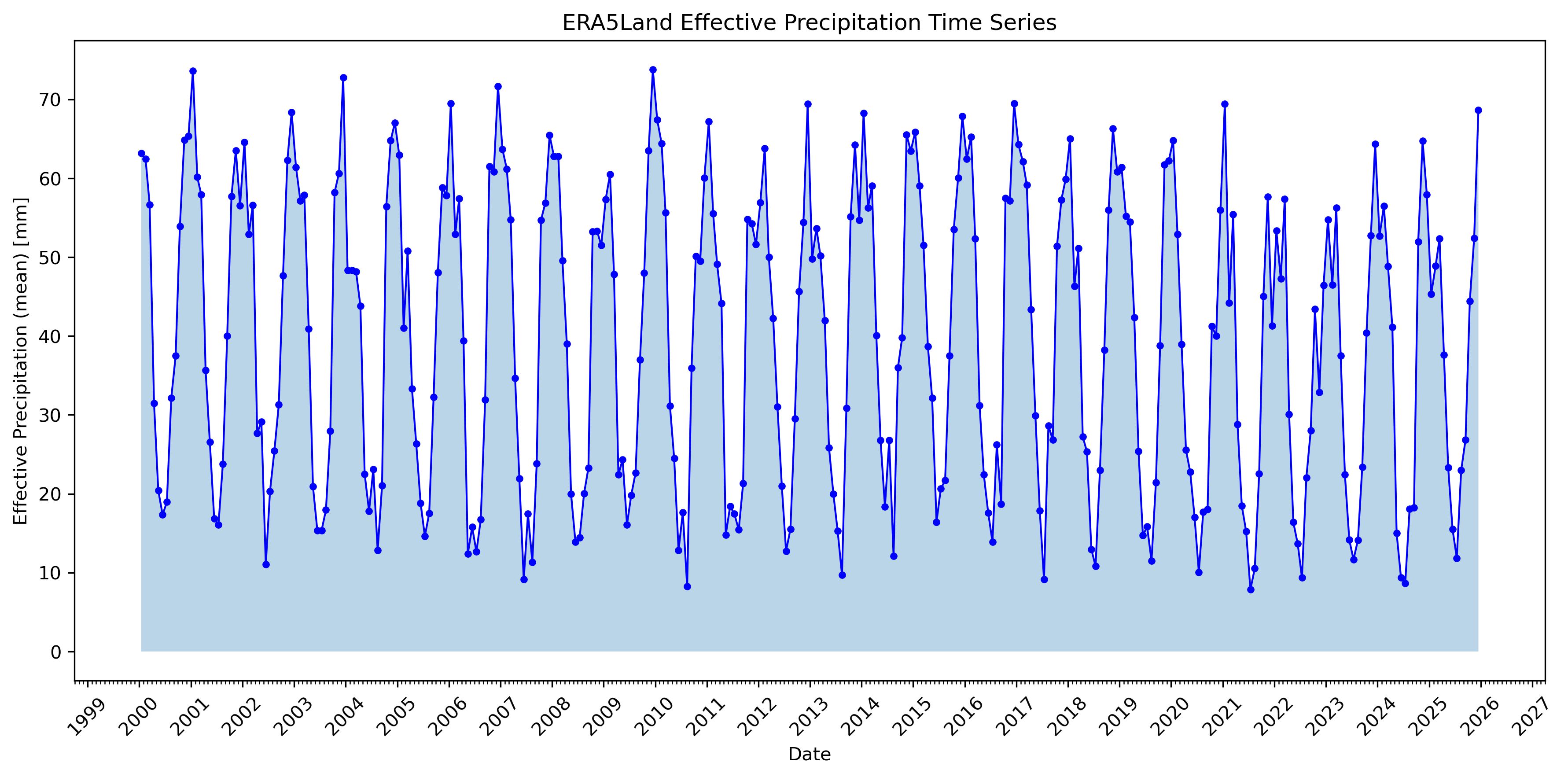
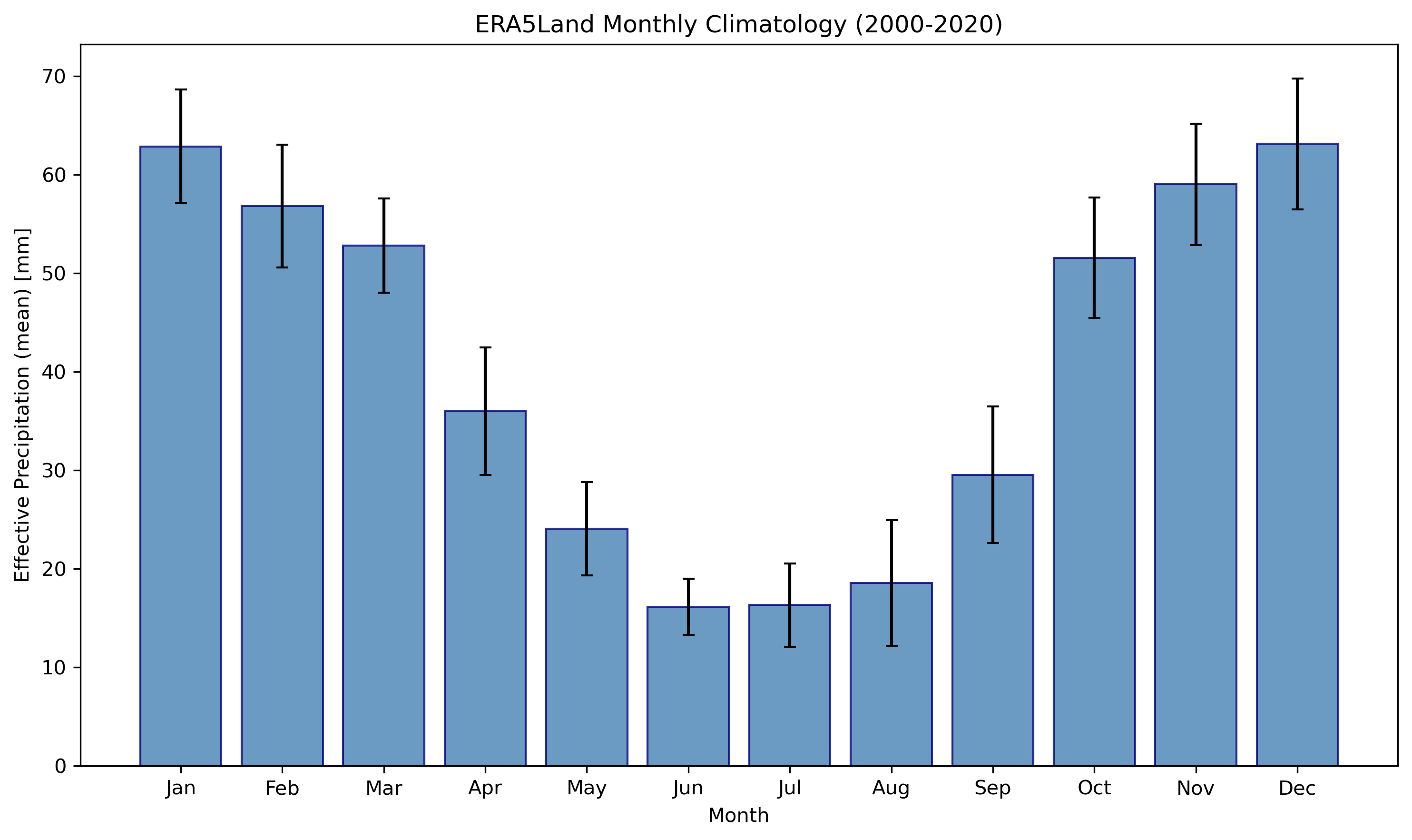
Left: Monthly effective precipitation time series (2000-2025). Right: Monthly climatology showing seasonal patterns.

Spatial Maps

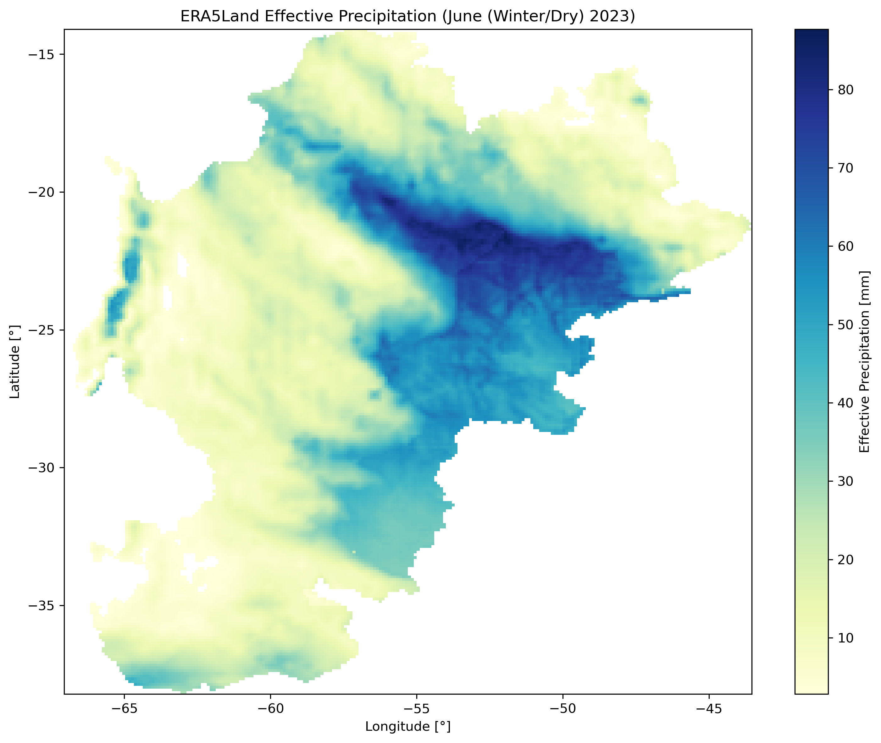
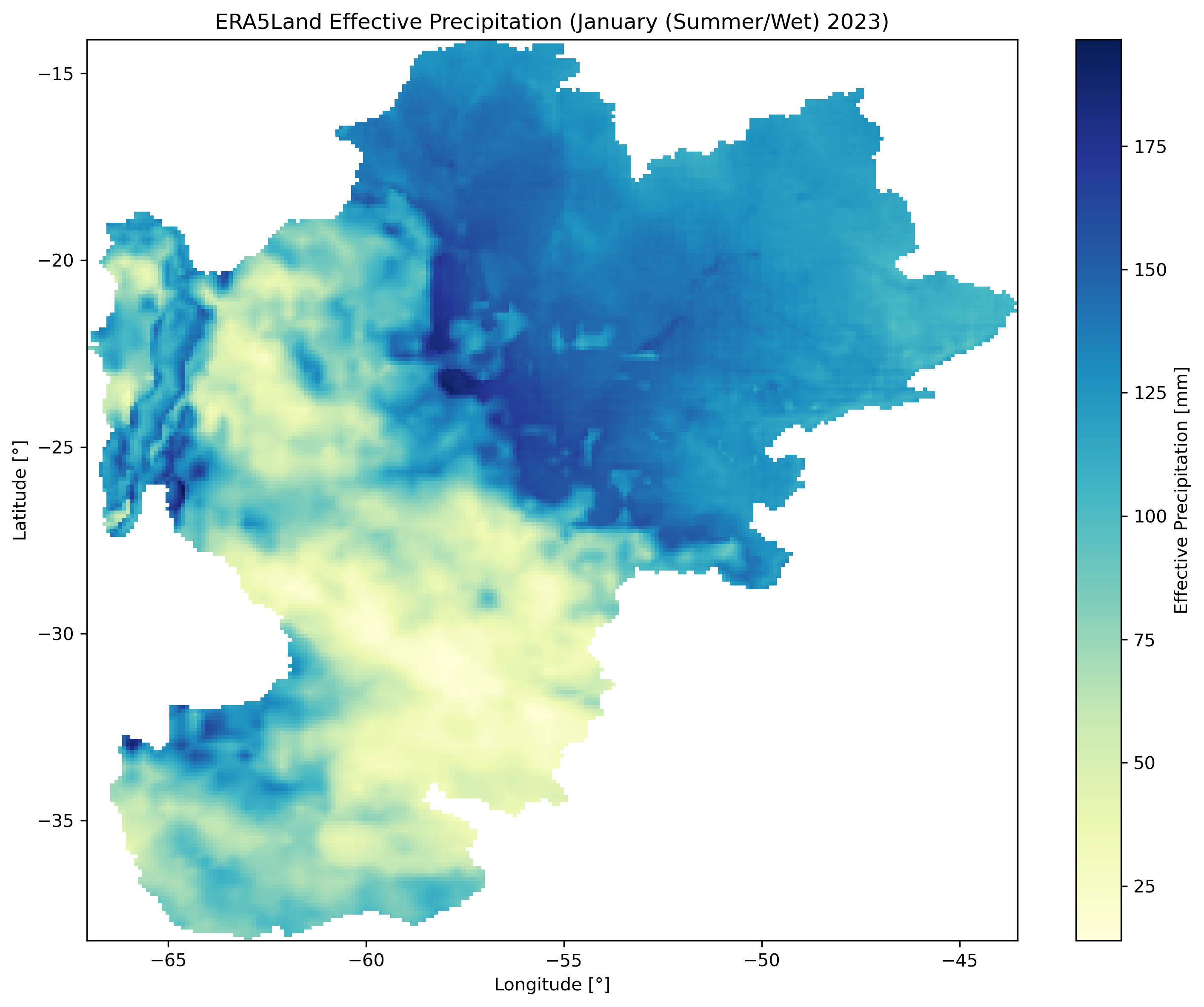
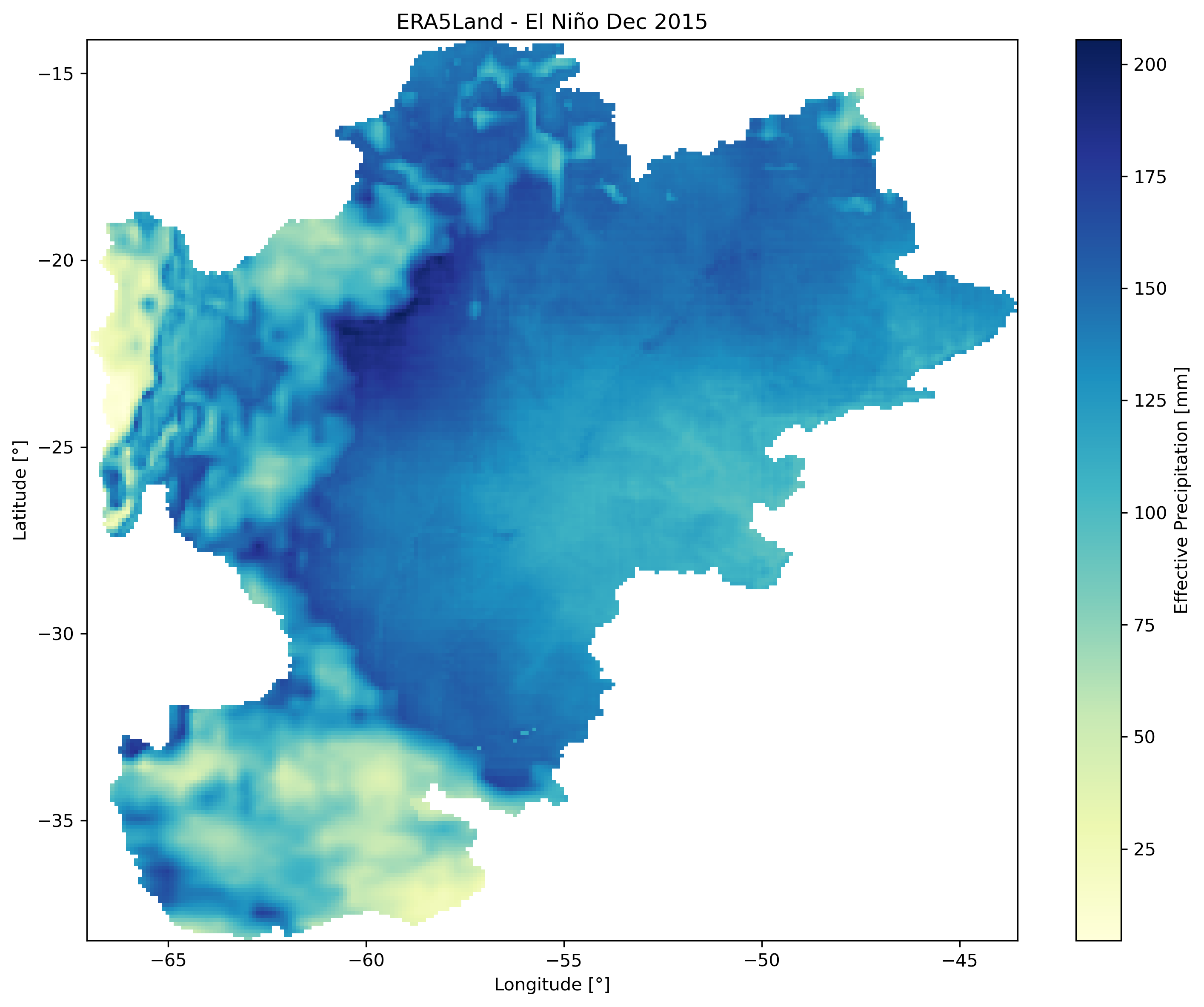
Left: Winter dry season (June 2023). Center: Summer wet season (January 2023). Right: El Niño event (December 2015).

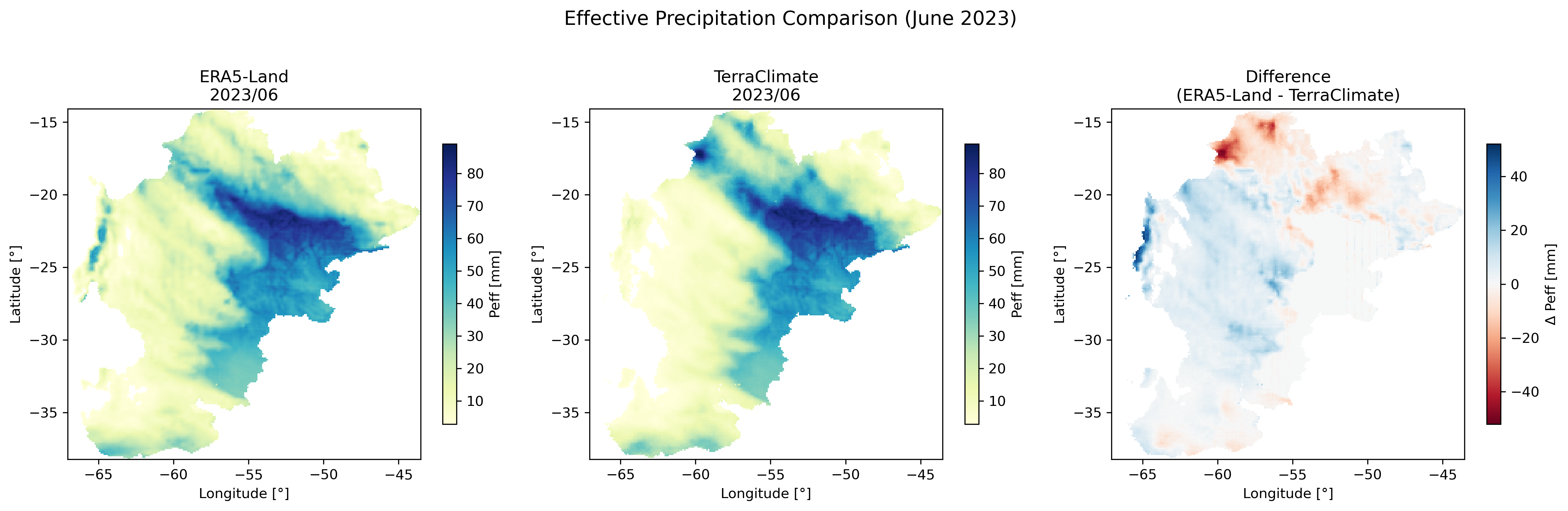
Dataset Comparison (ERA5-Land vs TerraClimate)

Side-by-side comparison of ERA5-Land and TerraClimate effective precipitation with difference map.

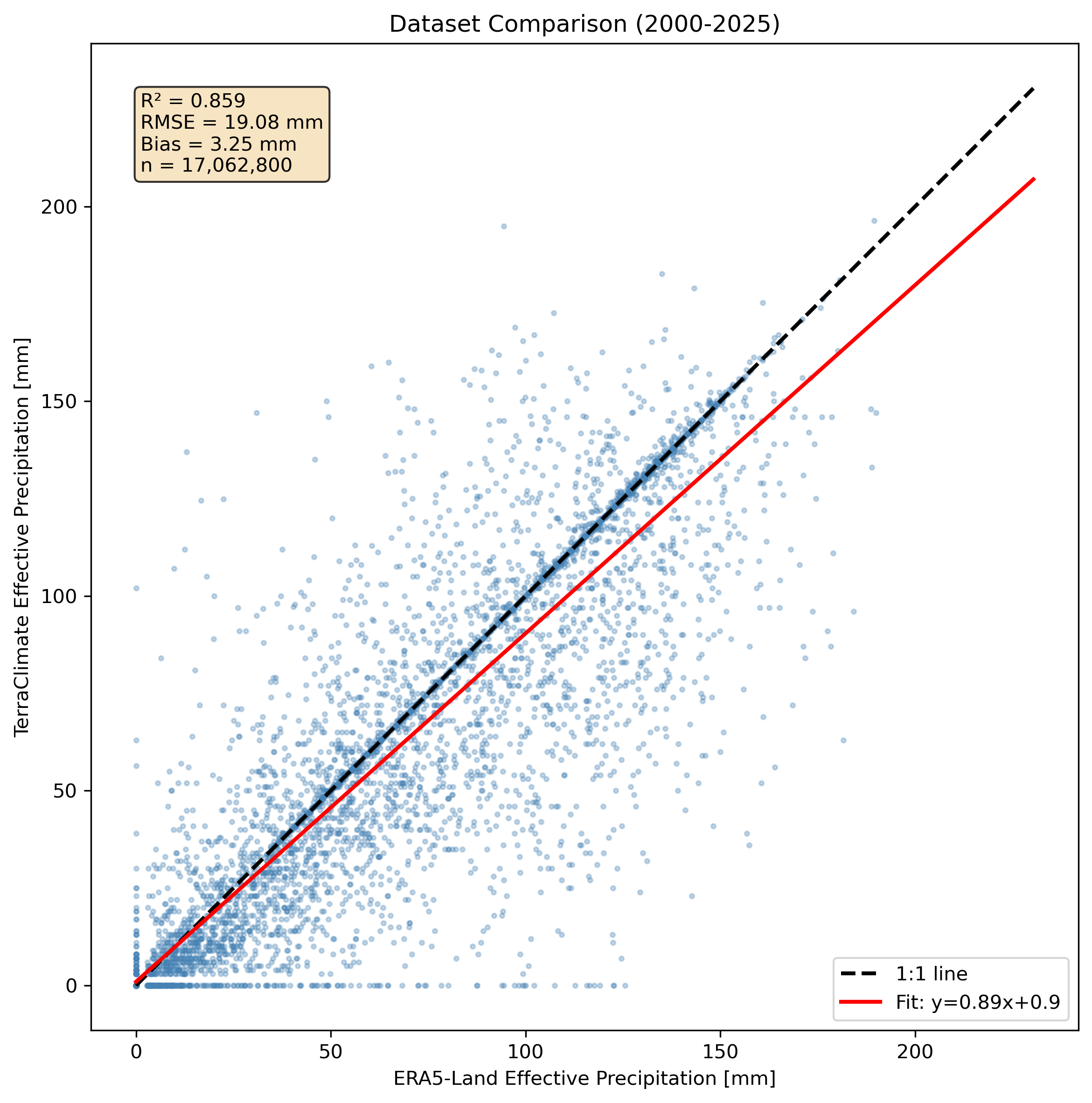
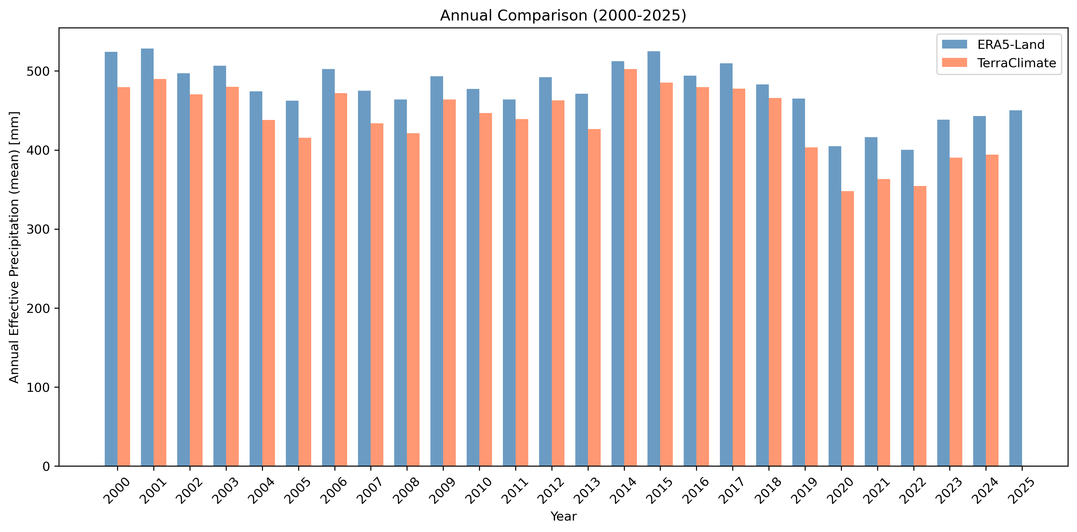
Left: Scatter plot comparison with R², RMSE, and bias statistics. Right: Annual totals comparison.

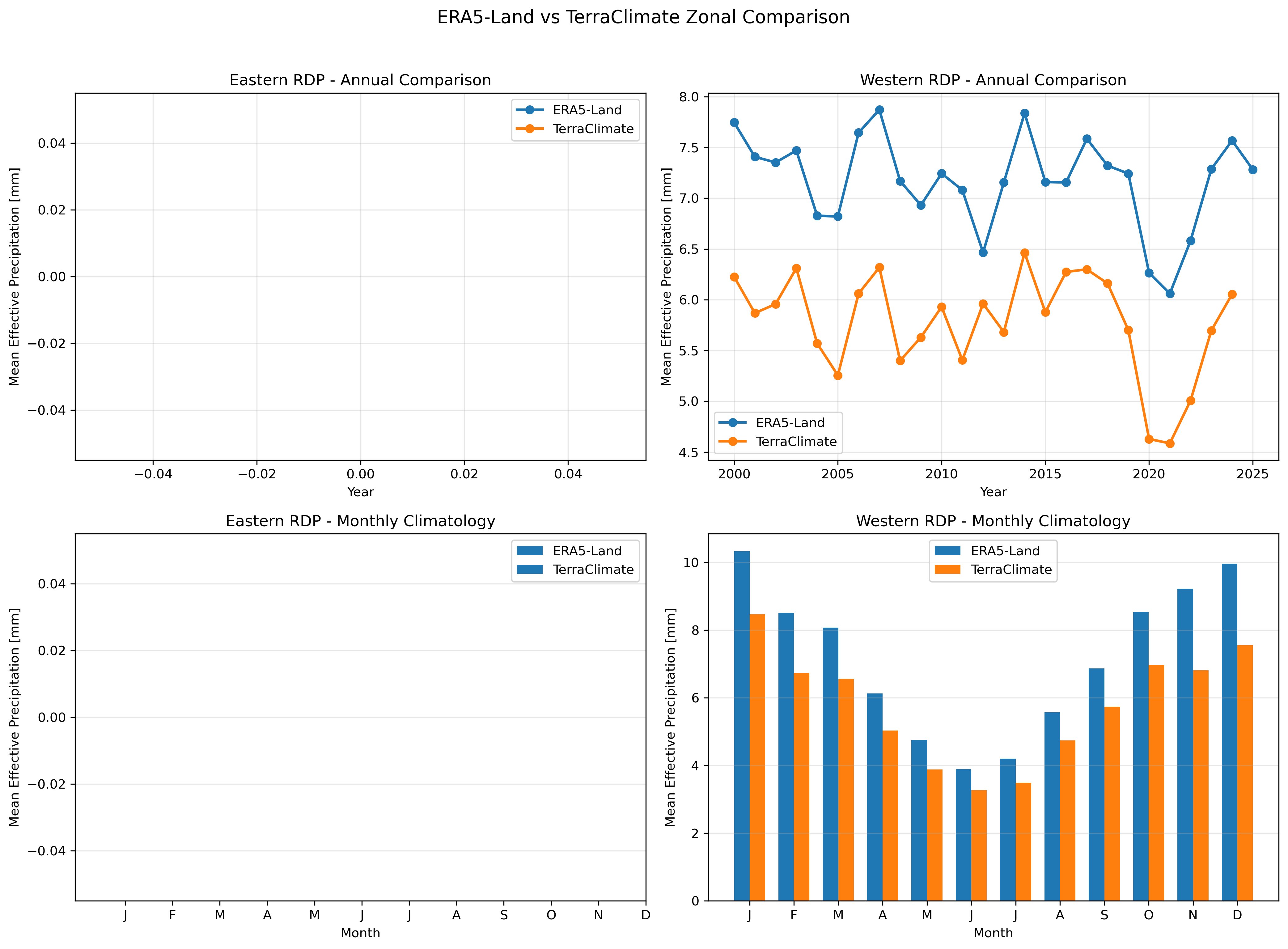
Zonal statistics comparison between ERA5-Land and TerraClimate for Eastern and Western Rio de la Plata regions.

Anomaly, Climatology & Trend Maps

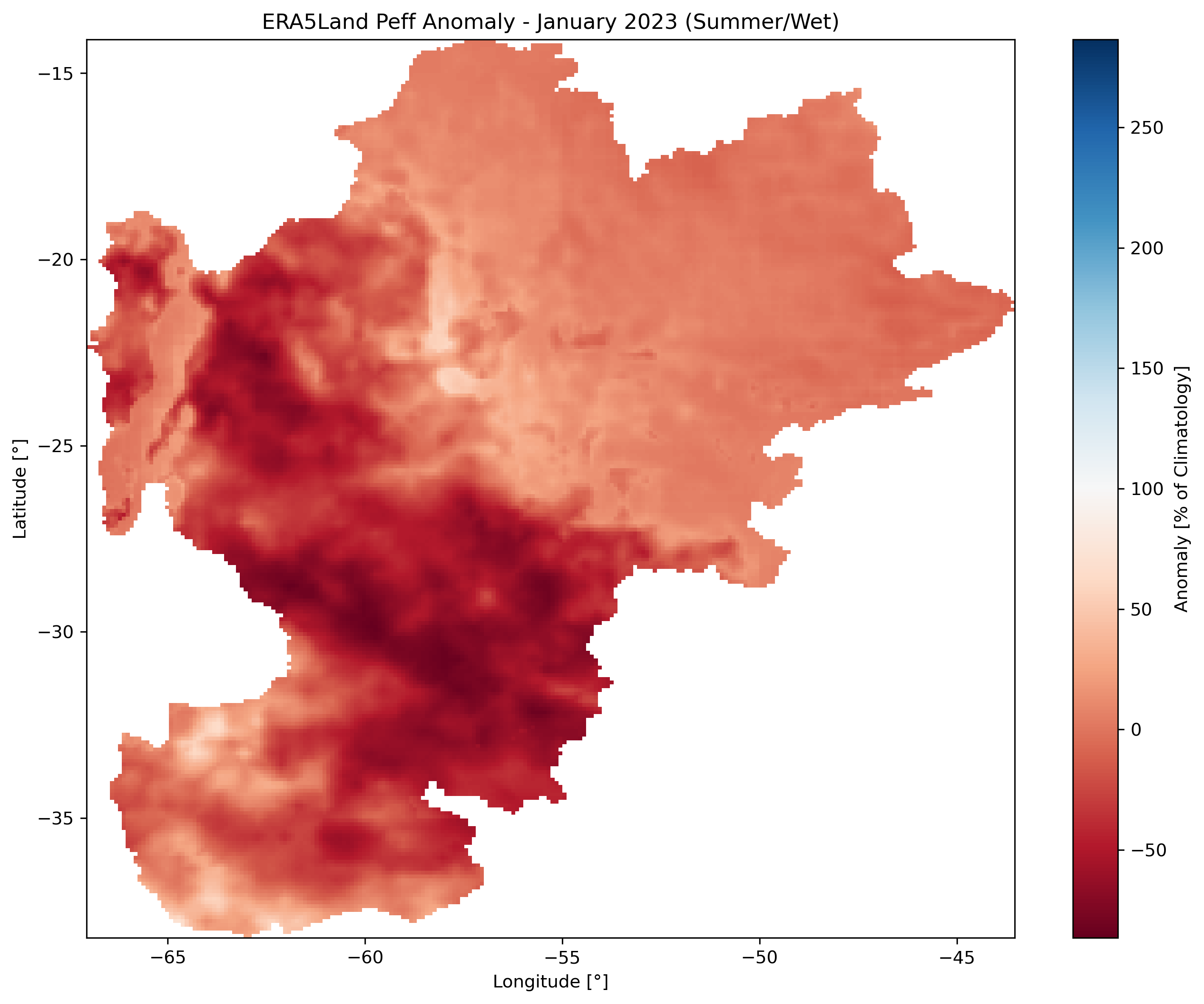
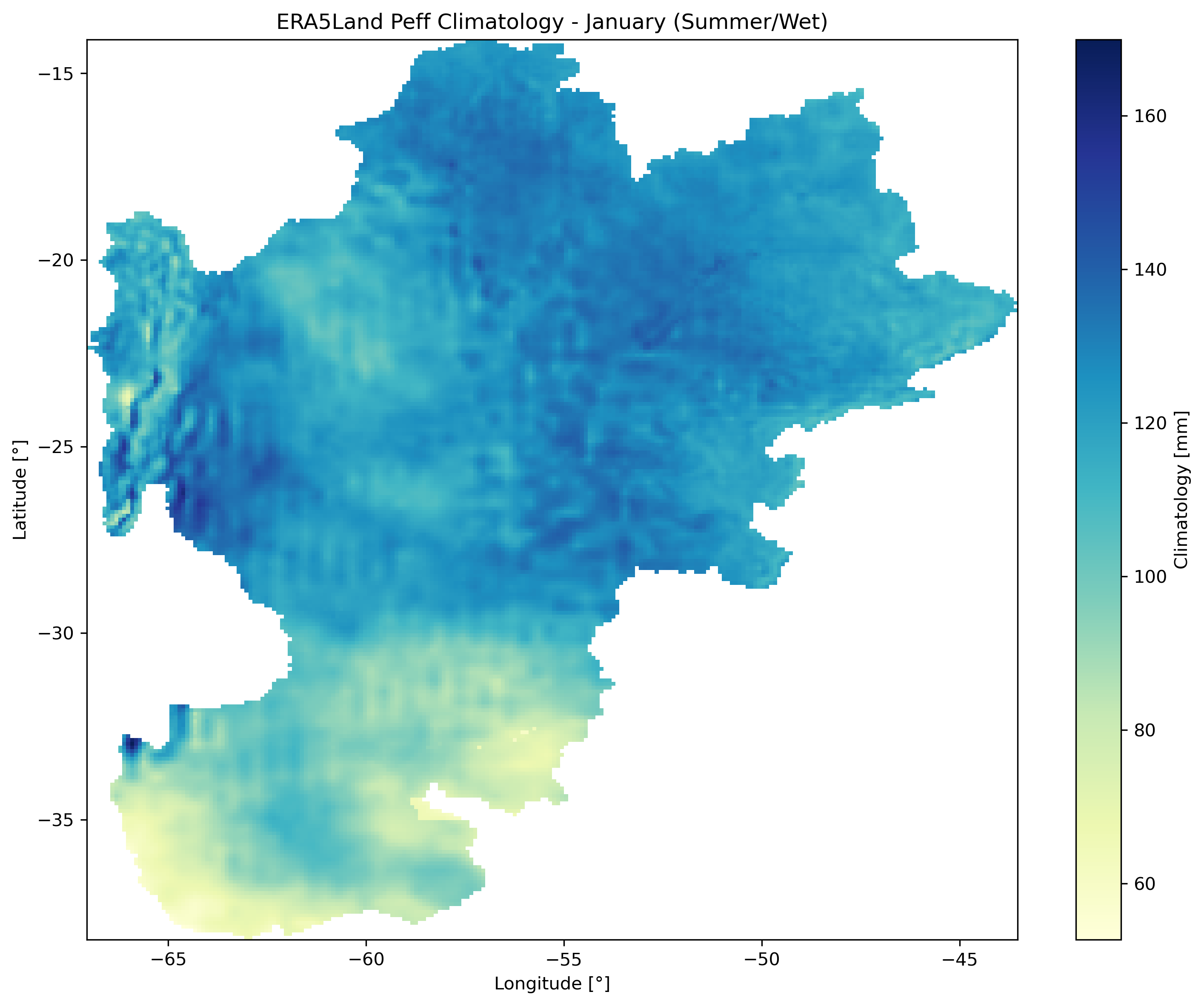
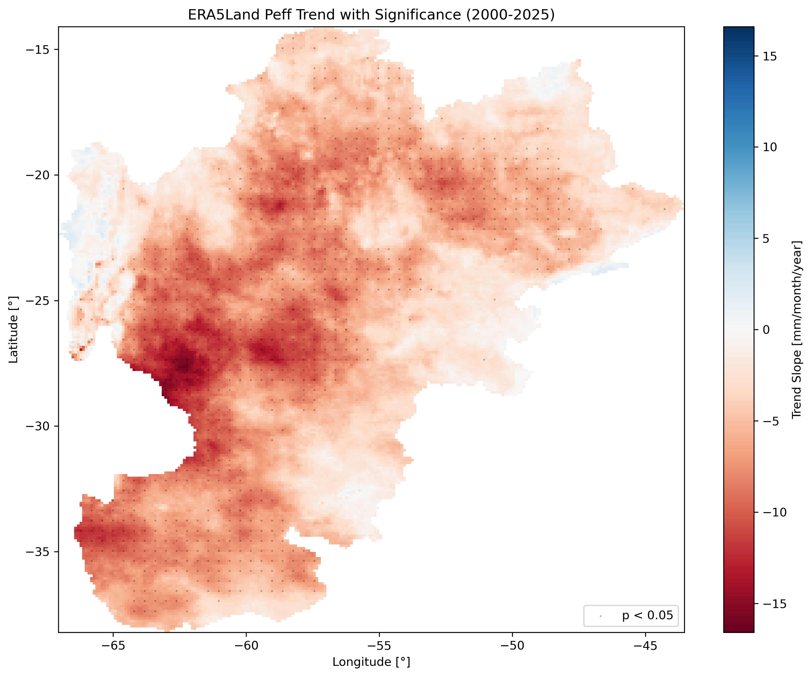
Left: Percent anomaly (January 2023). Center: January climatology (2000-2020). Right: Long-term trend with significance stippling (p < 0.05).

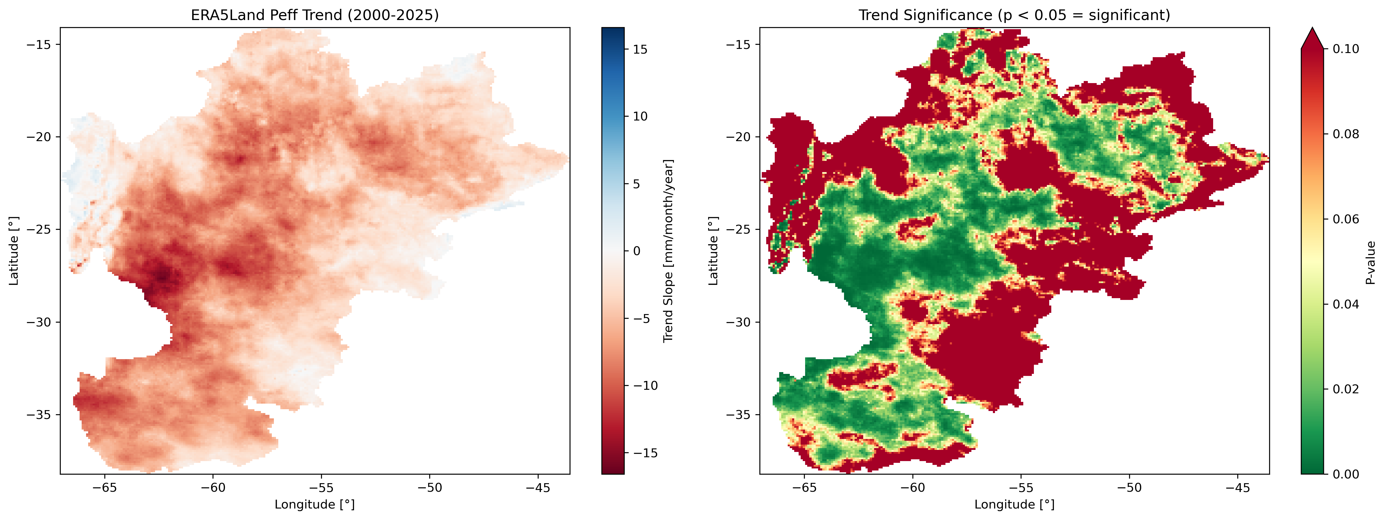
Trend analysis panel showing slope (mm/year) and p-value maps side by side.

Method Comparison

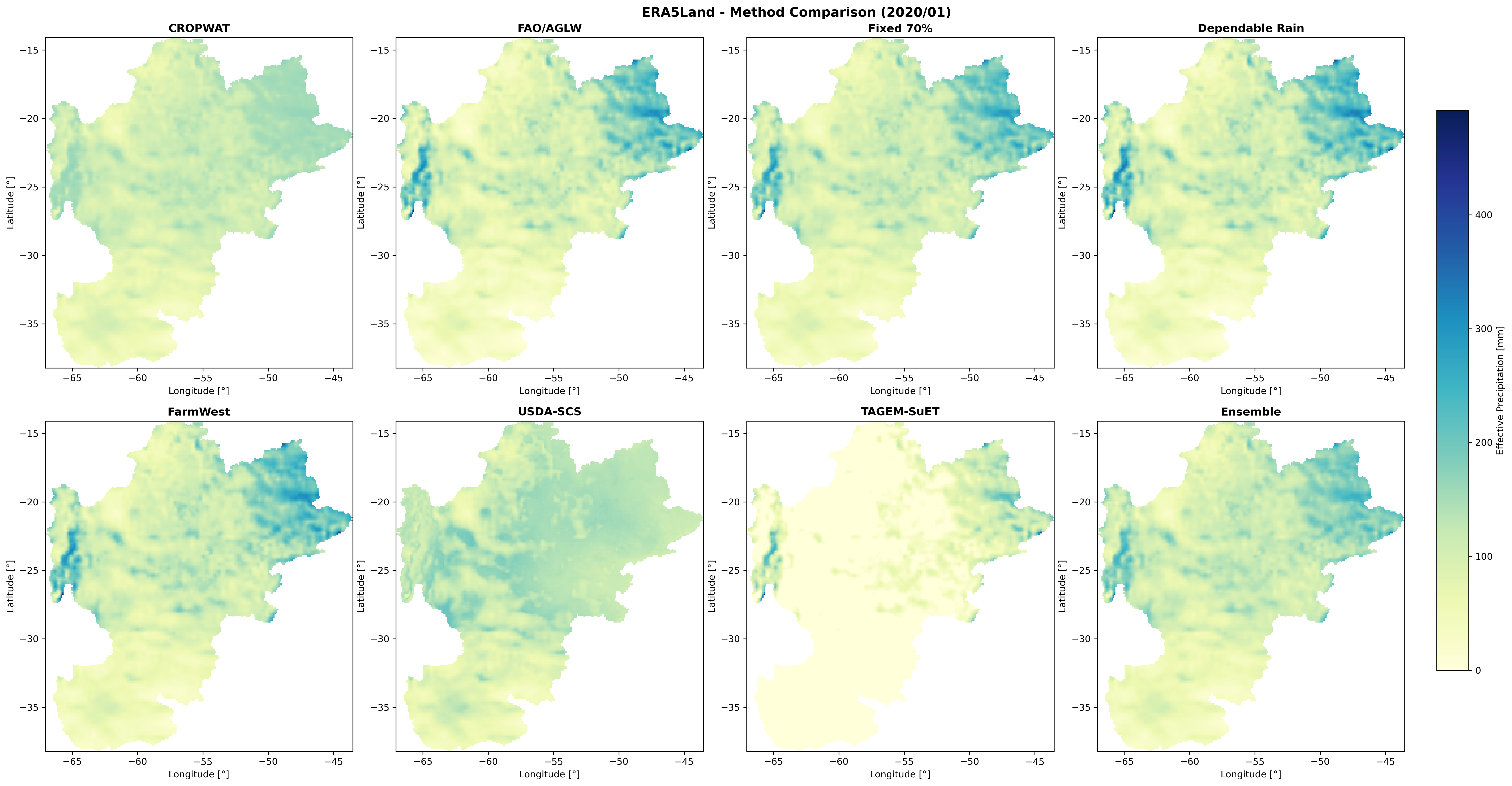
Comparison of 8 effective precipitation methods: CROPWAT, FAO/AGLW, Fixed Percentage (70%), Dependable Rainfall (80%), FarmWest, USDA-SCS, TAGEM-SuET, and Ensemble.

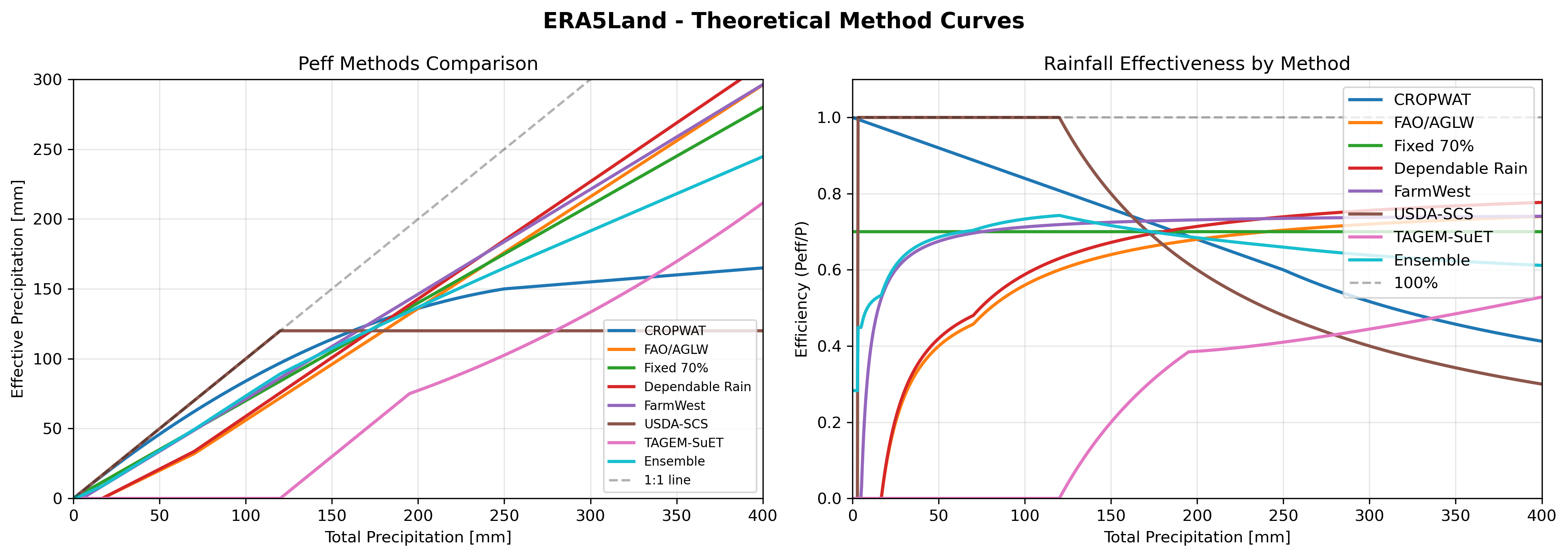
Theoretical response curves for different effective precipitation methods.

Arizona USDA-SCS Example Outputs

The Arizona workflow (Examples/arizona_example.py) demonstrates U.S.-specific datasets with the USDA-SCS method:

Time Series & Climatology

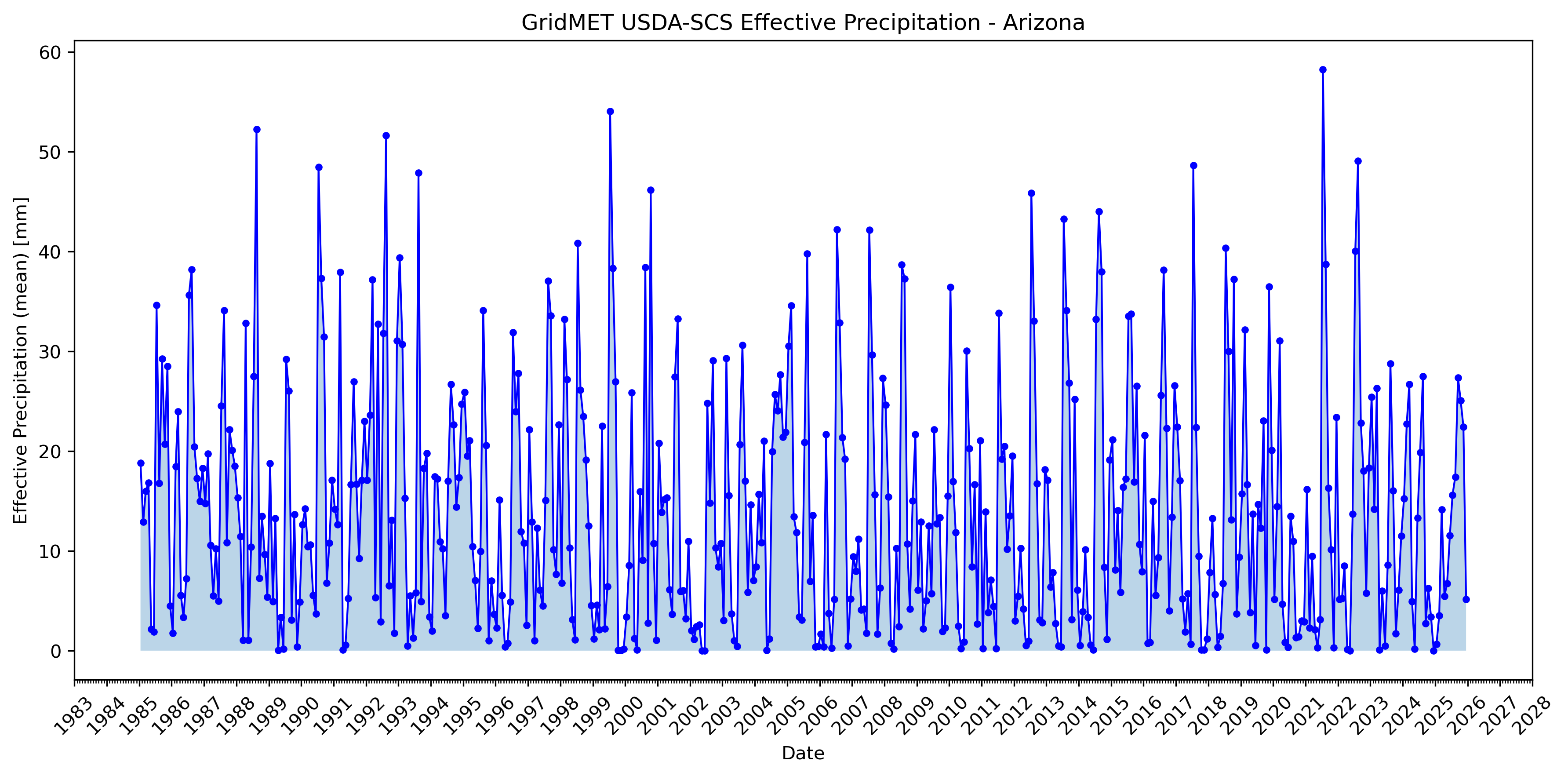
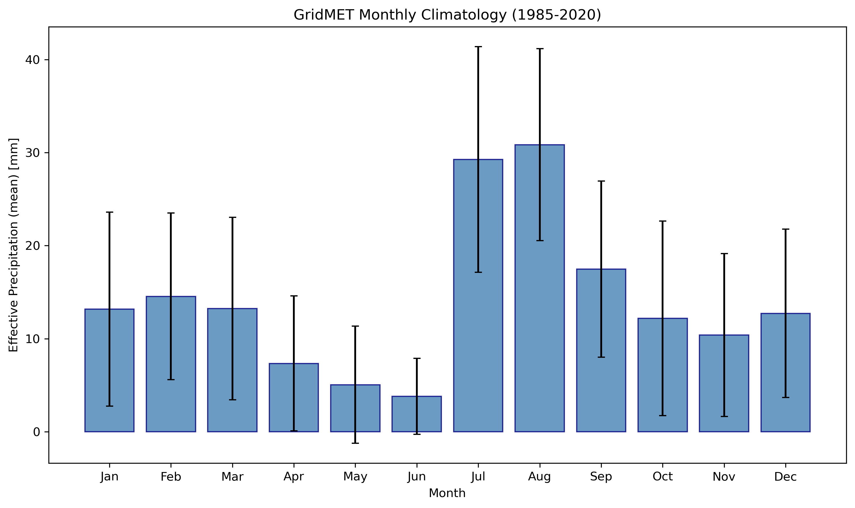
GridMET USDA-SCS effective precipitation for Arizona: time series (left) and monthly climatology (right).

Anomaly, Climatology & Trend Maps

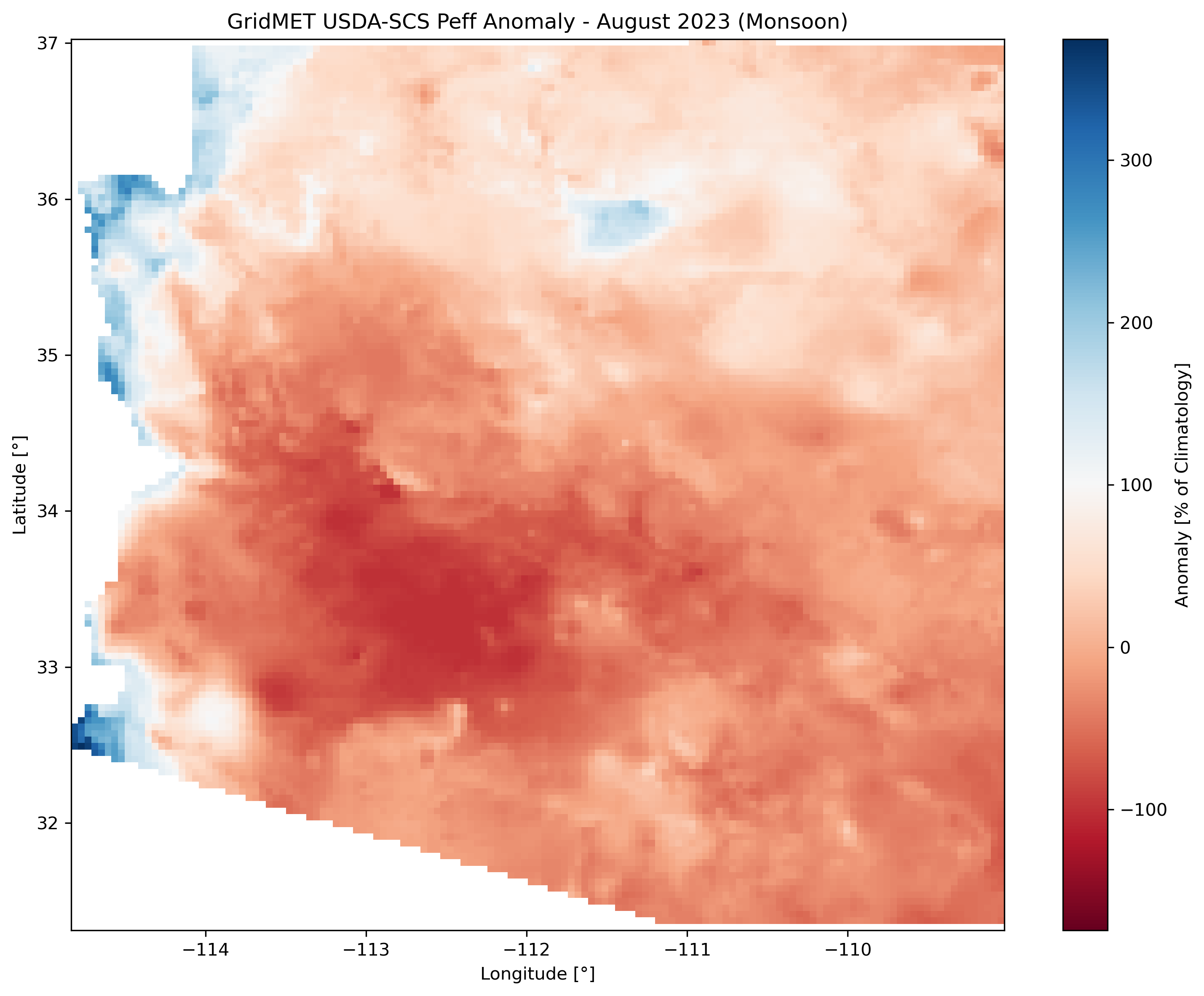
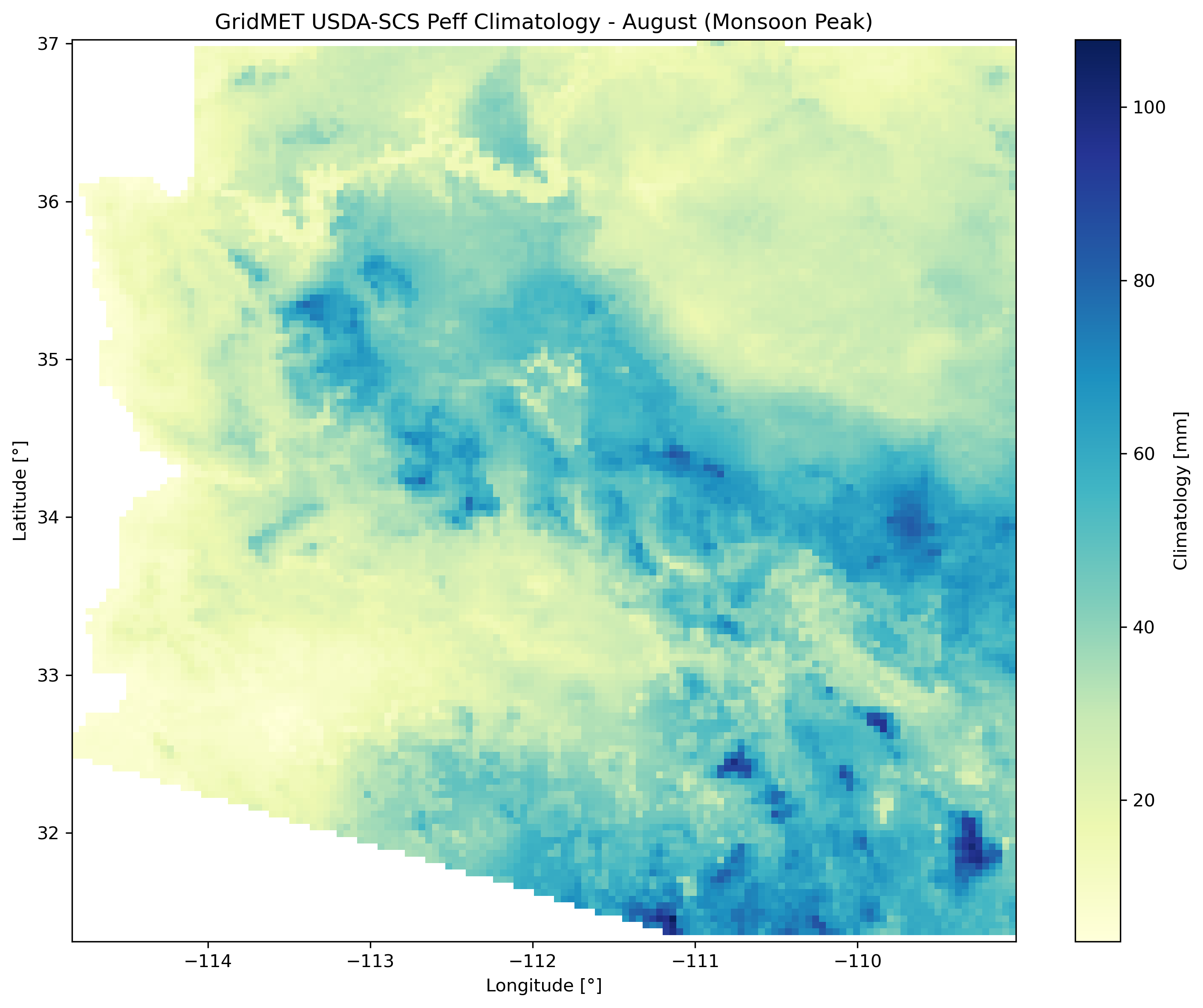
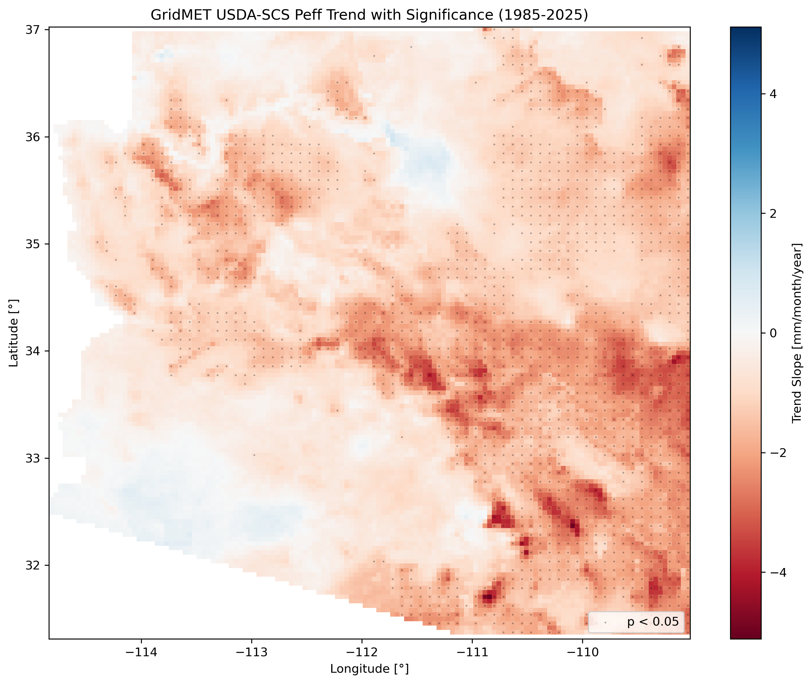
Left: August 2023 anomaly (monsoon season). Center: August climatology (monsoon peak). Right: Long-term trend with significance stippling.

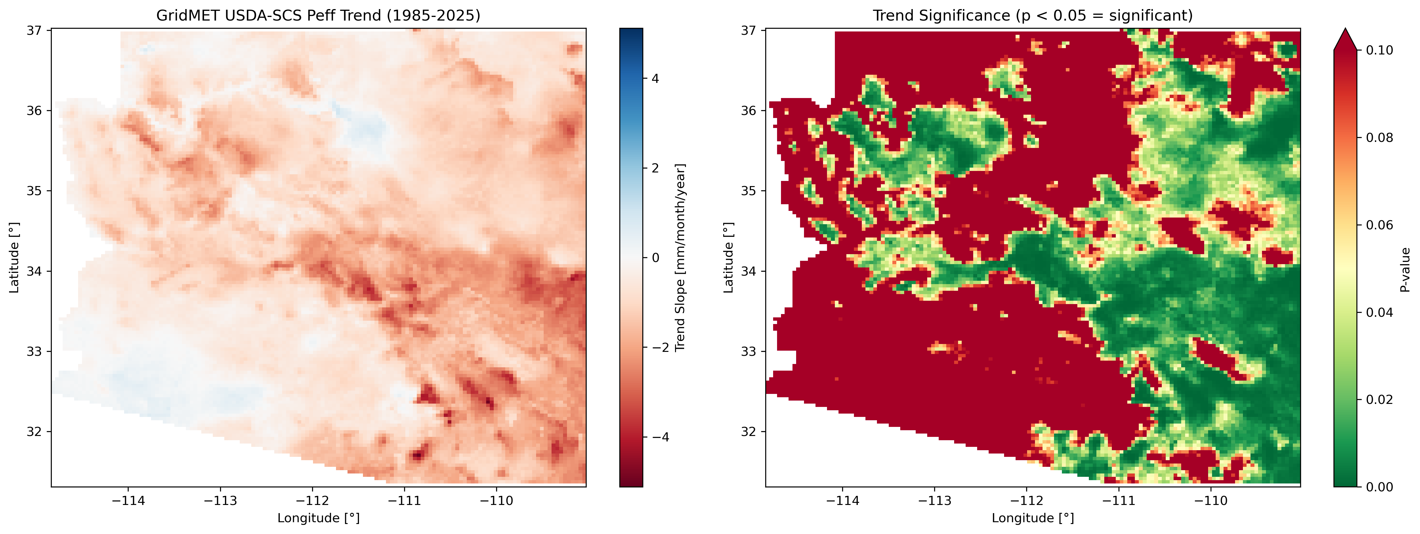
Trend analysis panel for Arizona showing slope and p-value maps.

U.S. vs Global Dataset Comparison

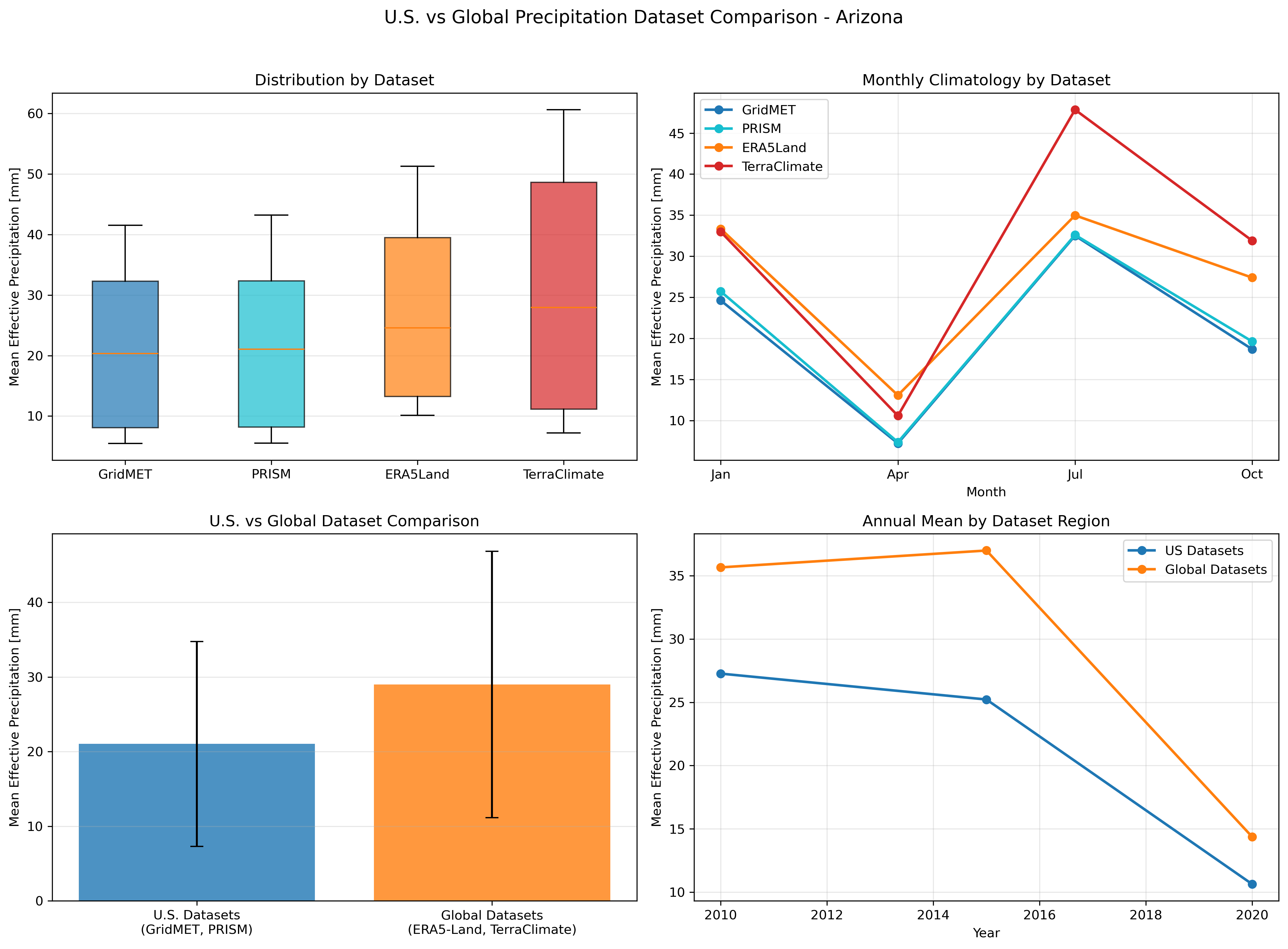
Comparison of U.S. datasets (GridMET, PRISM) vs Global datasets (ERA5-Land, TerraClimate) for Arizona.

New Mexico 8-Method Comparison Example Outputs

The New Mexico workflow (Examples/new_mexico_example.py) compares 8 effective precipitation methods using PRISM data (excludes PCML):

Mean Annual Comparison (1986-2025)

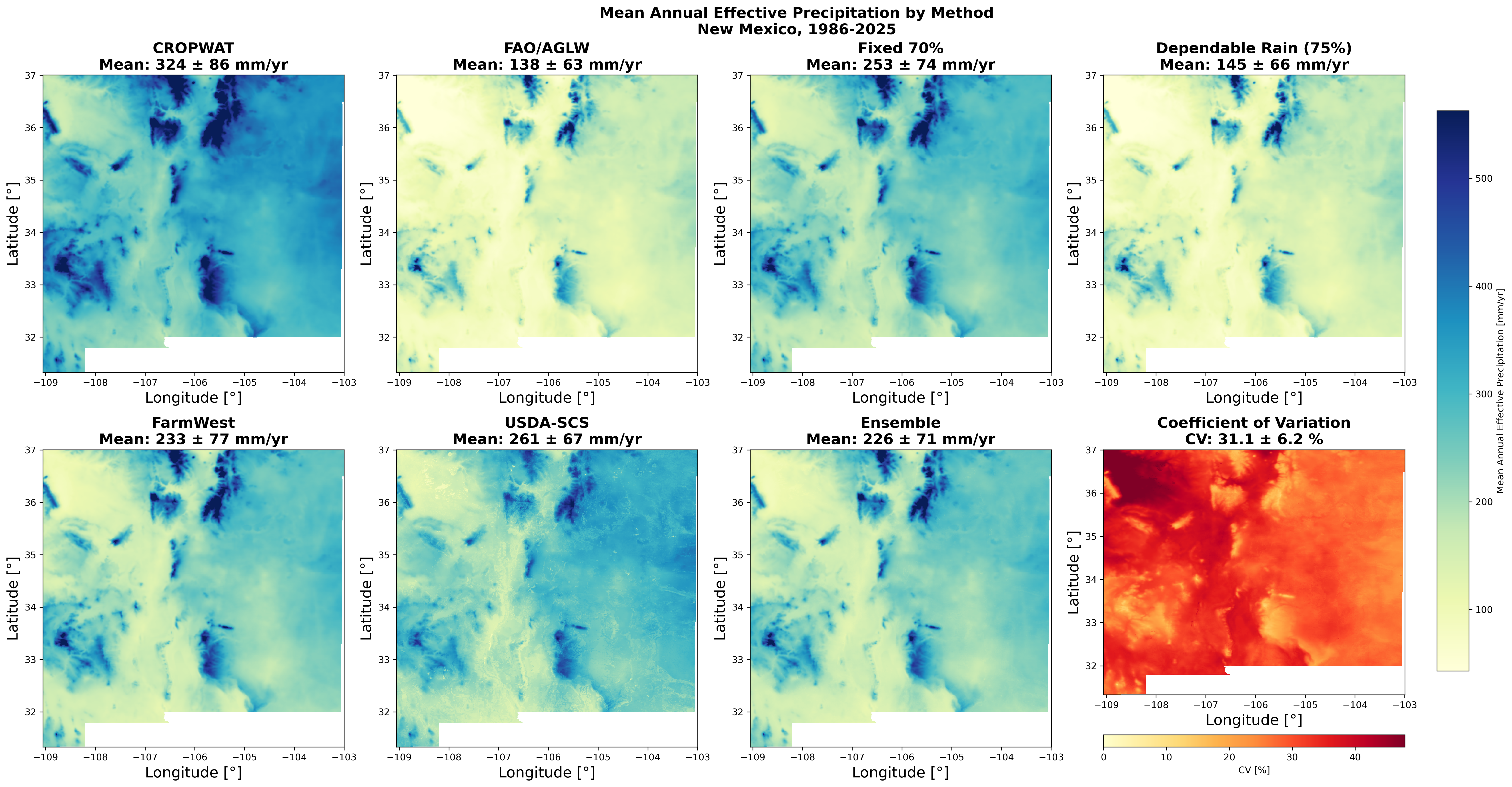
Mean annual effective precipitation (1986-2025) for 8 methods: CROPWAT, FAO/AGLW, Fixed 70%, Dependable Rainfall, FarmWest, USDA-SCS, TAGEM-SuET, and Ensemble.

Method Curves

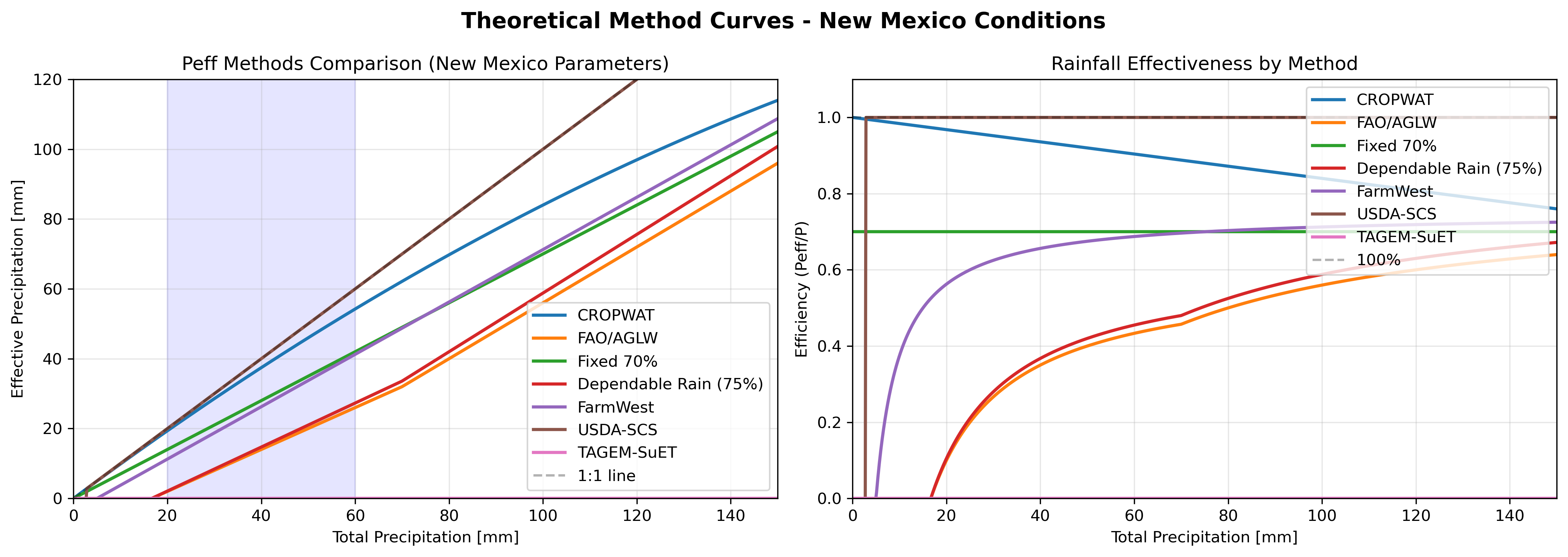
Theoretical response curves for 8 effective precipitation methods using New Mexico typical values (AWC=120mm/m, ETo=200mm/month).

Western U.S. PCML Example Outputs

The Western U.S. PCML workflow (Examples/western_us_pcml_example.py) demonstrates the Physics-Constrained Machine Learning method for the entire Western United States:

Summary Figure

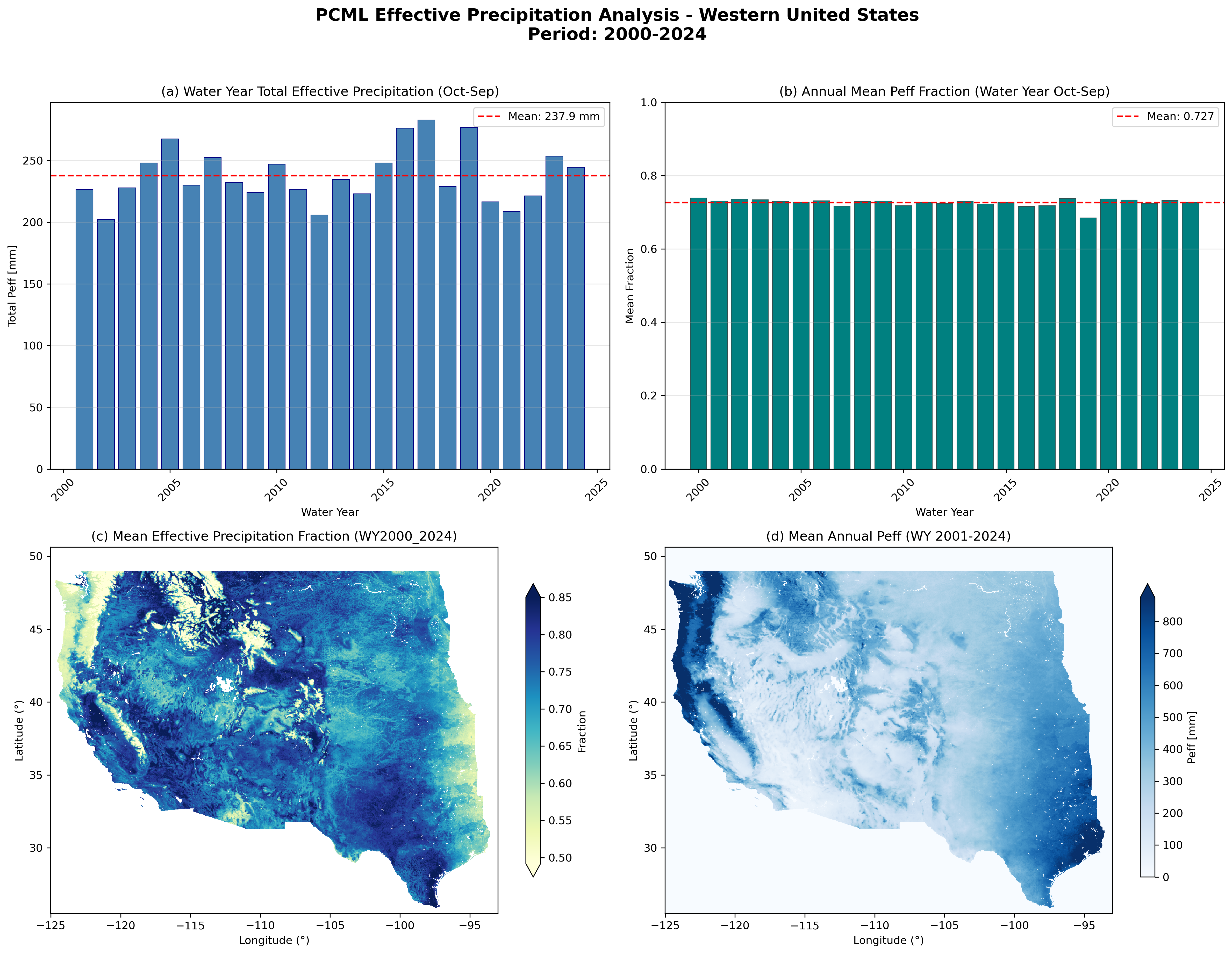
Summary of PCML effective precipitation analysis for the Western U.S. (WY 2001-2024): (a) Water year total time series, (b) Annual mean fraction time series, (c) Mean effective precipitation fraction map, (d) Mean annual effective precipitation map.

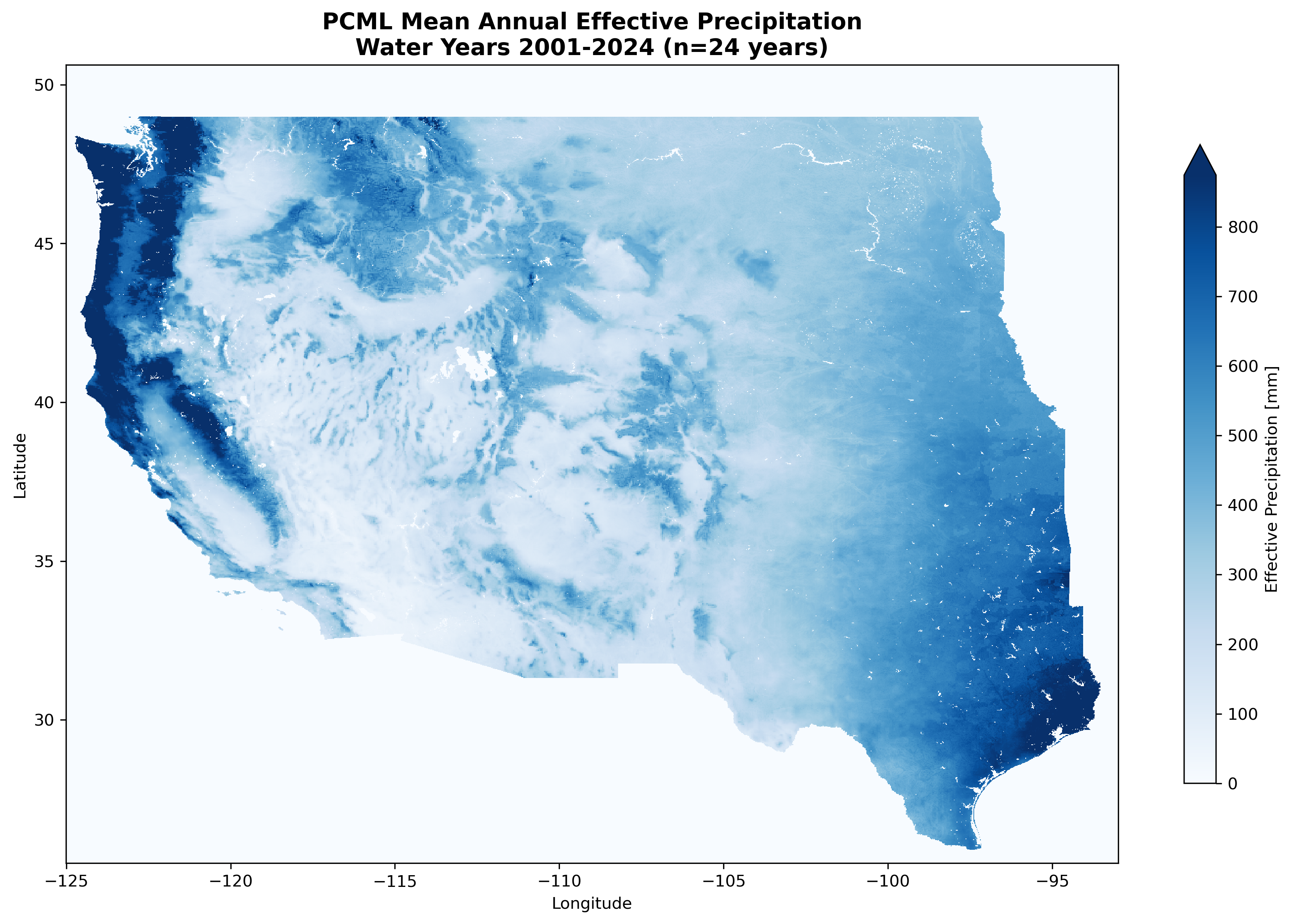
Mean Annual Effective Precipitation

Mean annual effective precipitation (WY 2001-2024) for the Western United States computed from the PCML GEE asset.

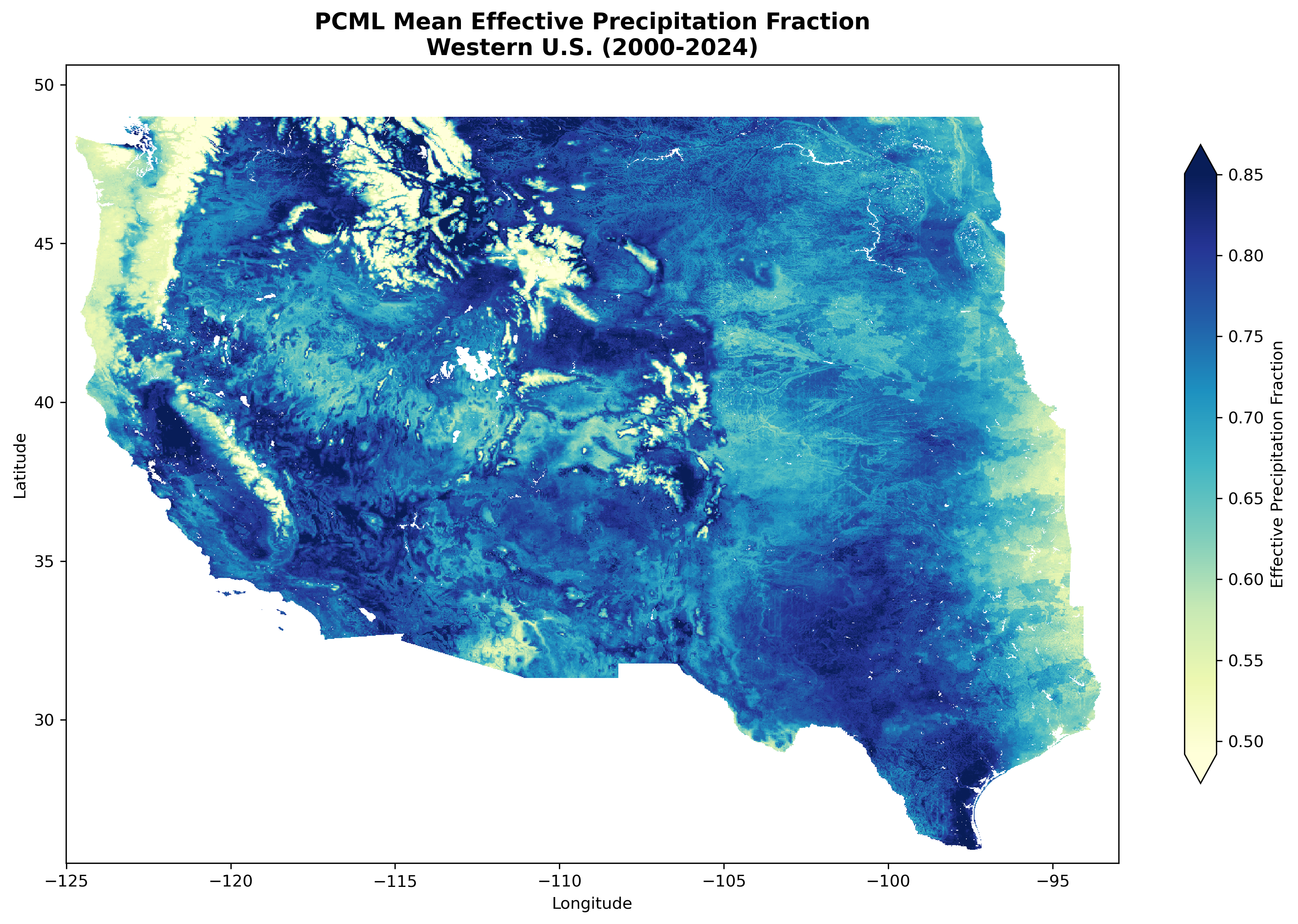
Mean Effective Precipitation Fraction

Mean annual effective precipitation fraction (Peff/Precip) for the Western United States (WY 2001-2024).

Field-Scale Aggregation (UCRB Example)

The Upper Colorado River Basin workflow (Examples/ucrb_example.py) demonstrates field-scale effective precipitation using existing precipitation volumes in a GeoPackage:

Key Features

No GEE precipitation download - Works with pre-existing monthly precipitation volumes
Field-level analysis - Individual agricultural parcels with unique identifiers
Zonal AWC statistics - Downloads SSURGO AWC data and calculates mean per field
Unit conversion - Handles acre-feet ↔ mm for method application
8 methods - CROPWAT, FAO/AGLW, Fixed 70%, Dependable Rain, FarmWest, and 3 USDA-SCS variants

Unit Conversion Workflow

Precipitation volume (acre-feet)
    → ÷ field area (acres) → depth (feet)
    → × 304.8 → depth (mm)
    → Apply pyCropWat method
    → ÷ 304.8 → depth (feet)
    → × field area (acres)
Effective precipitation volume (acre-feet)

Python API Example

import numpy as np
from pycropwat.methods import cropwat_effective_precip

# Convert acre-feet volume to mm depth
FT_TO_MM = 304.8
ppt_mm = (ppt_volume_acft / area_acres) * FT_TO_MM

# Apply pyCropWat method
peff_mm = cropwat_effective_precip(ppt_mm)

# Convert back to volume
peff_acft = (peff_mm / FT_TO_MM) * area_acres

For more examples and detailed API usage, see the Examples documentation.

Google Earth Engine Authentication

Before using pyCropWat, authenticate with Google Earth Engine:

earthengine authenticate

Or in Python:

import ee
ee.Authenticate()
ee.Initialize(project='your-project-id')

Citation

If you use pyCropWat in your research, please cite:

@software{pycropwat,
  author = {Majumdar, Sayantan and ReVelle, Peter and Pearson, Christopher and Nozari, Soheil and Minor, Blake A. and Hasan, M. F. and Huntington, Justin L. and Smith, Ryan G.},
  title = {pyCropWat: A Python Package for Computing Effective Precipitation Using Google Earth Engine Climate Data},
  year = {2026},
  url = {https://github.com/montimaj/pyCropWat},
  doi = {10.5281/zenodo.18201619}
}

Effective Precipitation Method References

Muratoglu, A., Bilgen, G. K., Angin, I., & Kodal, S. (2023). Performance analyses of effective rainfall estimation methods for accurate quantification of agricultural water footprint. Water Research, 238, 120011. https://doi.org/10.1016/j.watres.2023.120011
Smith, M. (1992). CROPWAT: A computer program for irrigation planning and management (FAO Irrigation and Drainage Paper No. 46). Food and Agriculture Organization of the United Nations. https://www.fao.org/sustainable-development-goals-helpdesk/champion/article-detail/cropwat/en

Funding

This work was supported by a U.S. Army Corps of Engineers grant (W912HZ25C0016) for the project "Improved Characterization of Groundwater Resources in Transboundary Watersheds using Satellite Data and Integrated Models."

Principal Investigator: Dr. Ryan Smith (Colorado State University)

Co-Principal Investigators:

Dr. Ryan Bailey (Colorado State University)
Dr. Justin Huntington (Desert Research Institute)
Dr. Sayantan Majumdar (Desert Research Institute)
Mr. Peter ReVelle (Desert Research Institute)

Research Scientist:

Dr. Soheil Nozari (Colorado State University)

Roadmap

The following features have been implemented or are under consideration for future releases:

✅ Implemented (v1)

📊 Temporal Aggregation

✅ Seasonal summaries (DJF, MAM, JJA, SON)
✅ Annual totals with statistics
✅ Growing season aggregations based on crop calendars
✅ Custom date range aggregations

📈 Statistical Analysis

✅ Long-term climatology (e.g., 30-year normals)
✅ Anomaly detection (absolute, percent, standardized)
✅ Trend analysis using linear regression or Theil-Sen/Mann-Kendall
✅ Zonal statistics for polygons

🔄 Additional Effective Precipitation Methods

✅ FAO/AGLW method
✅ Fixed percentage method (configurable percentage)
✅ Dependable rainfall (FAO method at different probability levels)
✅ FarmWest method (Pacific Northwest irrigation)
✅ USDA-SCS method (soil moisture depletion with AWC and ETo)
✅ TAGEM-SuET method (P - ETo with 75mm cap)
✅ PCML method (Physics-Constrained ML for Western U.S., Jan 2000 - Sep 2024)
✅ Ensemble method (mean of 6 methods, excludes TAGEM-SuET and PCML)

📁 Example Workflows

✅ South America example (Rio de la Plata, 8 methods)
✅ Arizona example (U.S. vs Global datasets, 8 methods)
✅ New Mexico example (PRISM with IrrMapper mask, 8 methods)
✅ Western U.S. PCML example (17 states, water year aggregation)
✅ UCRB field-scale example (GeoPackage with AWC lookup)

📤 Enhanced Export Options

✅ NetCDF output for time-series analysis
✅ Cloud-Optimized GeoTIFFs (COGs)
✅ Zonal statistics CSV export by polygon

📉 Visualization

✅ Built-in plotting functions for time series
✅ Monthly climatology bar charts
✅ Raster map visualization
✅ Interactive maps (folium/leafmap integration)
✅ Comparison plots between datasets (side-by-side, scatter, annual)

🚧 Planned for Future Releases

🌾 Crop Water Requirements

Crop coefficient (Kc) integration for different crop types/stages
Net irrigation requirement (ETc - Peff) calculations
Crop calendar support for region-specific growing seasons

📈 Advanced Analysis

Drought indices (SPI, SPEI) integration
Direct cloud storage export (GCS, S3)

✅ Validation Tools

Station data comparison module
Cross-dataset validation (e.g., ERA5 vs TerraClimate)
Uncertainty quantification

💧 Water Balance Extension

Evapotranspiration integration (from MODIS, SSEBop, OpenET)
Simple water balance (P - ET - Runoff)

Have a feature request? Please submit your ideas via GitHub Issues. We welcome community contributions and feedback!

License

This project is licensed under the MIT License - see the LICENSE file for details.

Name		Name	Last commit message	Last commit date
Latest commit History 87 Commits
.github/workflows		.github/workflows
Examples		Examples
docs		docs
pycropwat		pycropwat
tests		tests
.gitignore		.gitignore
CHANGELOG.md		CHANGELOG.md
LICENSE		LICENSE
MANIFEST.in		MANIFEST.in
README.md		README.md
environment.yml		environment.yml
mkdocs.yml		mkdocs.yml
pyproject.toml		pyproject.toml
requirements.txt		requirements.txt

License

montimaj/pyCropWat

Folders and files

Latest commit

History

Repository files navigation

pyCropWat

Project Structure

Overview

Effective Precipitation Methods

CROPWAT

FAO/AGLW Formula (Dependable Rainfall)

Fixed Percentage Method

Dependable Rainfall Method

FarmWest Method

USDA-SCS Method (with AWC and ETo)

TAGEM-SuET Method (with ETo)

PCML (Physics-Constrained Machine Learning)

Ensemble - Default (Mean of Methods)

Method Comparison

Installation

Quick Install (PyPI)

Disk Space Requirements

Using Conda (Recommended for Development)

From Source (pip)

Usage

Python API

Temporal Aggregation & Analysis

Export Options

Command Line Interface

Process Command Examples

Aggregate Command Examples

Analyze Command Examples

Export Command Examples

Plot Command Examples

CLI Arguments

Global Options

Process Command Arguments

Output Files

Output Resolution

Large Region Handling

Important: Units

Temporal Aggregation

Common GEE Climate Assets

Global Precipitation Datasets

U.S.-Specific Precipitation Datasets

USDA-SCS Method Required Datasets

Complete Workflow Examples

1. Rio de la Plata Basin Example (Global)

What the Example Does

Running the Example

Configuration

2. Arizona USDA-SCS Example (U.S.)

USDA-SCS Method Configuration

What the Example Does

Running the Example

CLI Equivalent

Configuration

Output Structure

Example Outputs

Time Series & Climatology

Spatial Maps

Dataset Comparison (ERA5-Land vs TerraClimate)

Anomaly, Climatology & Trend Maps

Method Comparison

Arizona USDA-SCS Example Outputs

Time Series & Climatology

Anomaly, Climatology & Trend Maps

U.S. vs Global Dataset Comparison

New Mexico 8-Method Comparison Example Outputs

Mean Annual Comparison (1986-2025)

Method Curves

Western U.S. PCML Example Outputs

Summary Figure

Mean Annual Effective Precipitation

Mean Effective Precipitation Fraction

Field-Scale Aggregation (UCRB Example)

Key Features

Unit Conversion Workflow

Python API Example

Packages